Duo Functions
This section shows examples of the definitions of the analytical functions supported in Duo.
Note
Duo function type names are case-insensitive in the input. In this manual we use the canonical
spelling shown in the section headings (typically uppercase) and format function names as LIKE_THIS.
Citations are given consistently as DOI links where available.
Potential energy functions
Extended Morse Oscillator EMO
 ,
,
which has the form of a Morse potential with a exponential tail and the distance-dependent exponent coefficient
beta_{rm EMO}(r) = sum_{i=0}^N a_i y_p^{rm eq}(r)^i,
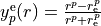
expressed as a simple power series in the reduced variable:
y_p^{rm e}(r) = frac{r^p-r_{rm e}^p}{r^p+r_{rm e}^p}
with  as a parameter. This form guarantees the correct dissociation limit and allows for extra flexibility in the degree of the polynomial on the left or on the right sides of a reference position
  which we take at
  . This is specified by the parameters
 (
( ) and
) and 
 (
( ),
respectively.
),
respectively.
Example:
poten 2
name "a 3Piu"
symmetry u
type  EMO
lambda 1
mult   3
values
Te          0.81769829519421E+03
Re          0.13115676812526E+01
Ae          0.50960000000000E+05
RREF       -0.10000000000000E+01
PL          4
PR          4
NL          2
NR          3
a0          0.21868146887665E+01
a1          0.88875855351916E-01
a2          0.84932592800179E-01
a3          0.23343175838290E+00
end
Taylor expansion around  :
:

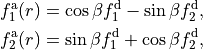
Morse Long-Range (MLR) function MLR

where the radial variable  in the exponent, the long-range potential
  by
by 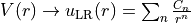 while the exponent coefficient function
![\beta_{\rm MLR}(r) = y_p^{\rm{ref}}(r)\, \beta_{\infty} + \left[1 -y_p^{\textrm{ref}}(r)\right] \sum_{i=0} a_i[y_q^{\textrm{ref}}(r)]^i](_images/math/aceee807e89ff6672ea54e2f3ab326b133a039d7.png)
is defined in terms of two radial variables which are similar to , but are defined with respect to a different expansion center r_textrm{ref}, and involve two different powers, and  . The above definition of the function
  means that:
![\beta_{\rm MLR}(r\to\infty) \equiv \beta_{\infty} = \ln[2D_{\rm e}/u_{\textrm{LR}}(r_{\rm e})].](_images/math/c7948f3dd437cd732ef5d3c93588cfaf62c60dfb.png)
Example:
poten 6
name "d 3Pig"
symmetry g
lambda 1
mult   3
type  MLR
values
  Te        0.20151357236994E+05
  RE        0.12398935933004E+01
  AE        0.50960000000000E+05        link   1   1   3
  RREF     -0.10000000000000E+01
  P         0.40000000000000E+01
  NL        0.20000000000000E+01
  NR        0.80000000000000E+01
  b0        0.30652655627150E+01
  b1       -0.93393246763924E+00
  b2        0.45686541184906E+01
  b3       -0.37637923145046E+01
  b4       -0.41028177891391E+01
  b5        0.00000000000000E+00
  b6        0.00000000000000E+00
  b7        0.00000000000000E+00
  b8        0.00000000000000E+00
  a1        0.00000000000000E+00
  a2        0.00000000000000E+00
  a3        0.00000000000000E+00
  a4        0.00000000000000E+00
  a5        0.00000000000000E+00
  a6        192774.
  a7        0.00000000000000E+00
  a8        0.00000000000000E+00
end
Coxon and Hajigeorgiou’s MLR3 Morse Long-Range with Douketis Damping MLR3
The MLR3 potential function is described by Coxon and Hajigeorgiou, JCP 132 (2010) - an adapted form of the standard MLR potential with an additional parameter  in the radial variable
  . The form of the potential is given by:

where Here,  is the minimu and the long-range potential function is given by:
Here Duo uses the generalised Douketis damping functions, defined as:
![D_n(r) = \left(1 - \exp \left[ - \frac{b(s) (\rho r)}{n} - \frac{c(s) (\rho r)^2}{\sqrt{n}} \right] \right)^{m+s}](_images/math/ec2c2f6e72ab8bffcca2890326f11a7ef8682acd.png)
with  where
where 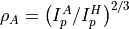 and
and  is the ionisation potential of the hydrogen atom. The
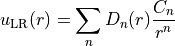
  function is given by:
![\phi_\text{MLR3} (r) = y_m(r, r_\text{ref}) \phi_\text{MLR3} (\infty) + \left[ 1 - y_m(r, r_\text{ref}) \right] \sum_{i=0}^{N_\phi} \phi_i y_q(r, r_\text{ref})^i](_images/math/2b6e6c56e4fd1a2101d4df5dba9e20c5818b7845.png)
where

where  is some expansion centre, usually
  .
.
Most parameters in the input file have a one-to-one correspondence with those in the above equations. The parameter V0 can be set greater than zero if the dissociation energy,  is not defined relative to the potential minimum (i.e
  ).
).
Further parameters that do not have obvious definitions are NPWRS and NPHIS. The former specifies the number of inverse power terms to include in the long-range function, and is followed by the order of each power term (in the example below, the first power term is  , the second is
  , etc.), the coefficients
  are then specified (
COEF1, COEF2, etc.). The parameter NPHIS specifies the number of  terms to include in the exponent function, and is followed by a list of their values.
An example input is given below for HF molecule. The parameters are taken from Coxon & Hajigeorgiou, JQSRT 151, 133–154 (2015).
poten 1
name "X1Sigma+"
symmetry +
lambda 0
mult 1
type MLR3
units cm-1 angstroms
values
V0      0.
RE      0.91683897
DE      49361.6
RREF    1.45
P       6
M       11
Q       4
A       150.0
S      -0.5
RHO     1.082
B       3.69
C       0.4
NPWRS   3
PWR1    6
PWR2    8
PWR3    10
COEF1   3.1755E+4
COEF2   1.667E+5
COEF3   1.125E+6
NPHIS   32
PHI0    3.54289281000000E+00
PHI1   -5.41984130000000E+00
PHI2   -8.86976500000000E+00
PHI3   -2.93722400000000E+01
PHI4   -4.32900400000000E+01
PHI5   -7.13177000000000E+01
PHI6   -7.77911700000000E+01
PHI7    6.71510000000000E+01
PHI8   -3.51437300000000E+02
PHI9   -4.62131060000000E+03
PHI10   6.72490000000000E+02
PHI11   5.81178370000000E+04
PHI12   1.90159300000000E+04
PHI13  -4.78435670000000E+05
PHI14  -3.29985590000000E+05
PHI15   2.60051860000000E+06
PHI16   2.52642570000000E+06
PHI17  -9.62119030000000E+06
PHI18  -1.17913360000000E+07
PHI19   2.41995750000000E+07
PHI20   3.62543670000000E+07
PHI21  -4.01790300000000E+07
PHI22  -7.51160300000000E+07
PHI23   4.00889000000000E+07
PHI24   1.03908000000000E+08
PHI25  -1.61464000000000E+07
PHI26  -9.20420000000000E+07
PHI27  -9.93600000000000E+06
PHI28   4.71800000000000E+07
PHI29   1.41000000000000E+07
PHI30  -1.06400000000000E+07
PHI31  -4.70000000000000E+06
end
Hajigeorgiou and Le Roy’s MLJ Morse/Lennard-Jones oscillator MLJ
- The MLJ potential function is described by Hajigeorgiou and R. J. Le Roy, J. Chem. Phys. 112, 3949 (2000) and
Coxon and Dickinson, J. Chem. Phys. 121, 9378–9388 (2004) in the radial variable
 . The form of the potential is given by:
![V(r) = V_e + (A_{e}-D_e) \left[1 - \left(\frac{R_e}{R}\right)^n \exp\left\{ -\phi(r) z(r, r_e)\right\}\right]^2,](_images/math/10e4820c068088dd3e8062e0fc6560bda51f57d0.png)
where
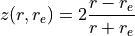
and
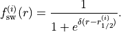
![\phi(r) = f_{\rm sw}(r) \sum_{m} \phi_m z^m + [1-f_{\rm sw}(r)] \phi_{\infty},](_images/math/4515cac7622ed5eb8e534f362aaca920250efb14.png)
with the switching function defined as:
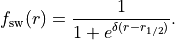
In case the long-range coefficient (leading term) is known,  can be estimated as
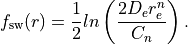
Otherwise it can be obtained through a fit.
An example input is given below for LiH molecule. The parameters are taken from Coxon and Dickinson, J. Chem. Phys. 121, 9378–9388 (2004)
poten X
name "X1Sigma+"
symmetry +
lambda 0
mult 1
type MLJ
values
TE           0.00000000000000E+00
RE           1.59559416124
AE           20286.0
R12          5.15
delta        2.25
phiinf       0.36722
N            6
phi0         -4.2014672169
phi1         0.80668167
phi2         0.11048407
phi3         0.5325794
phi4         0.379195
phi5         0.25342
phi6         0.24914
phi7         2.0402
phi8         -1.0855
phi9         -9.2553
phi10        14.2154
phi11        12.6523
phi12        -34.8674
phi13        15.7635
end
Diagonal BO-breakdown functions (rotationless) BOB-Z-M-SWITCH, BOB_Z_M_SWITCH
This form is taken from Coxon and Dickinson, J. Chem. Phys. 121, 9378–9388 (2004). The BOB diabatic potential is given by:
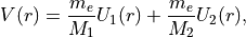
where
![U_i(r) = f^{(i)}_{\rm sw}(r) \sum_{m=1} u_m^{(i)} z^m + u_{\infty}^{(i)} \left[1-\frac{ f^{(i)}_{\rm sw}(r) }{f^{(i)}_{\rm sw}(r_e)}\right] ,](_images/math/5d92ccd5bfea73e5ff902237cb545fe37fada58a.png)
with the switching function defined as:
An example input for BOB-Z-M-SWITCH for LiH molecule is given by
diabatic X X
name "X1Sigma+"
symmetry +
lambda 0
mult 1.0
type BOB-Z-M-SWITCH
values
RE           1.59559416124
R12          5.0
delta        2.5
mass_Li      7.016003436590
Uinf_Li      0.0
N            2
U1           -0.77132e-4
U2           6.13522e-4
R12          5.25
delta        2.5
mass_H       1.007825032230
Uinf_H       -21145.50636
N            5
U1         -1.0229927e-5
U2         1.513 1552e-5
U3         -1.47383e-5
U4         1.39309e-5
U5         -0.67490e-5
end
The parameters are taken from Coxon and Dickinson, J. Chem. Phys. 121, 9378–9388 (2004)
Potential function Marquardt
 ,
,
which has the form of a Morse potential with a exponential tail and the distance-dependent damped exponent coefficient
:math:` Y(r) left( 1 - expleft{-beta_{rm M}(r) (r-r_{rm e})right} right) f_{rm Damp}(r) `
 ,
,
expressed as a simple power series in the reduced variable:
with as a parameter. The damping function is give by

Example:
poten 2
name "a 3Piu"
symmetry u
type  Marquardt
lambda 1
mult   3
values
Te          0.81769829519421E+03
Re          0.13115676812526E+01
Ae          0.50960000000000E+05
RREF       -0.10000000000000E+01
PL          4
PR          4
NL          2
NR          3
eps6        2.0
eps8        1.0
rs          1.0
a0          0.21868146887665E+01
a1          0.88875855351916E-01
a2          0.84932592800179E-01
a3          0.23343175838290E+00
end
Taylor expansion around :
Morse oscillator Morse
A polynomial expansion in the Morse variable 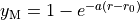 is used

Example
poten 1
name "X 1Sigmag+"
symmetry g +
type   MORSE
lambda 0
mult   1
values
TE             0.00000000000000E+00
RE             0.12423216077595E+01
a              0.20372796052933E+01
AE             0.73955889175514E+05
A1            -0.62744302960091E+04
A2            -0.57683579529693E+04
end
Morse_damp

Example:
poten 6
name "d 3Pig"
symmetry g
lambda 1
mult   3
type  Morse_damp
values
 Te      20121.09769
 re      0.12545760270976E+01
 Ae      0.50937907750000E+05        link   1   1   3
 a0      0.30398932686950E+01
 DAMP    0.10000000000000E-02
 a1      0.11437702960146E+05
 a2     -0.36585731834570E+03
 a3     -0.20920472718062E+05
 a4      0.90487097982036E-03
 a5      0.00000000000000E+00
 a6      0.00000000000000E+00
 a7      0.00000000000000E+00
 a8      0.00000000000000E+00
end
Modified-Morse
Alias MMorse
![V_(r)=T_{\rm e}+ (A_{\rm e}-T_{\rm e}) \frac{ \left[ 1-\exp\left(-\sum_{i=0} a_i \xi^{i+1}\right) \right]^2}{\left[ 1-\exp\left(-\sum_{i=0} a_i \right) \right]^2},](_images/math/aeab5f05713fa7ffa2bba3813916e2a3155783c4.png)
where  .
.
Example:
poten 8
name "Bp 1Sigmag+"
symmetry g +
lambda 0
mult   1
type  MMorse
values
Te            1.5408840263E+04
rE            1.3778208709E+00
Ae            5.0937907750E+04       link   1   1   3
a0            6.2733066935E+00
a1            1.4954972843E+01
a2            4.5160872659E+01
end
where the value  is ‘linked’ to the corresponding value of
 poten 1.
Polynomial
This keyword selects a polynomial expansion in the variable 

Example:
spin-orbit  2 2
name "<+1,S=1 (a3Pi)|LSZ|+1  (a3Pi),S=1>"
spin   1.0 1.0
sigma  1.0 1.0
lambda 1 1
type  polynom
factor   1
values
a0           14.97
re           1.3
a1           0.0
end
Taylor expansion around :

Dunham expansion
Dunham selects a polynomial expansion in the Dunham variable 

Example:
poten 1
name "X 2 Delta"
lambda 2
mult   2 type   Dunham values
Te              0.00000
Re              1.4399282269779912
a0         123727.20496894409      (= omega**2 / 4 B)
a2             -2.31
a3              3.80
a4             -6.00
a5              5.00
end
Taylor expansion around :

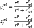
Simons, Parr and Finlan SPF
SPF selects a polynomial expansion in the the so-called Simons, Parr and Finlan variable 

Example:
poten 1
name "X 2Sigma+"
symmetry +
type   SPF
lambda 0
mult   2
values
Te         0.00000000000000E+00
RE         0.16292698613903E+01
a1         0.37922070444743E+06
a2         0.00000000000000E+00
a3        -0.53314483965665E+01
a4         0.00000000000000E+00
a5         0.19407192336518E+02
a4         0.00000000000000E+00
a5        -0.17800496953835E+03
end
Taylor expansion around :


where  is the maximum exponent included in the expansion. For long the potential goes to a constant value; convergence to the constant
is of the
is the maximum exponent included in the expansion. For long the potential goes to a constant value; convergence to the constant
is of the  type (correct for ions but too slow for neutral molecules).
Behaviour for 
The coefficient  is definitely positive, but
  can be positive and negative, so that
  can go to
  for short .
Murrell-Sorbie M-S
 `
where
`
where  .
.
Example:
poten 4
name "B 2Sigma"
symmetry -
type  M-S  (Murrell-Sorbie)
lambda 0
mult   2
values
V0            21000.0
RE            1.6
DE            25653.27131
a1            2.81468
a2            1.68719
a3            0.757787
a4            -0.5963168
a5            -0.54596343
a6            0.20611664
end
Taylor expansion around :

Behaviour for  :
:
 `
where is the maximum exponent included in the expansion. For long the potential goes to the constant value
`
where is the maximum exponent included in the expansion. For long the potential goes to the constant value  , and the asymptotic behavior is determined by the coefficients of the term with the highest exponent.
Chebyshev
This keyword selects an expansion in Chebyshev polynomials in the variable ![y= [r-(b+a)/2]/[(b-a)/2]](_images/math/54e0ce56743bc2440343f4581db2efd320fd759e.png) . The scaled variable ranges from
. The scaled variable ranges from  to 1 for in
 ![[a,b]](_images/math/b17897287b23d96473a85f41eeb859a16830b679.png) . The expansion is
. The expansion is

Example:
spin-orbit  2 2
name "<+1,S=1 (a3Pi)|LSZ|+1  (a3Pi),S=1>"
spin   1.0 1.0
type  chebyshev
factor   1
values
   a               0.80000000000000E+00
   b               0.26500000000000E+01
   A0             -0.25881057805341E+02
   A1              0.82258425882627E+01
   A2              0.52391700137878E+00
   A3              0.28483394288286E+01
   A4             -0.15136422837793E+00
   A5              0.97553692867070E-01
   A6             -0.25825811071417E+00
   A7             -0.69105144347567E-01
   A8             -0.44700771508442E-01
   A9              0.11793957297111E-01
   A10             0.16403055376257E-01
   A11             0.92509900186428E-02
   A12             0.50789943150707E-02
   A13            -0.39439903216016E-03
end
irreg_chebyshev_DMC
based on eq.(3) of https://doi.org/10.1016/j.jqsrt.2022.108255
COSH-POLY
This function can be used as a coupling for a diabatic representation of potentials characterised by an avoiding crossing and is given by:
Example
diabatic  1 8
name "<X1Sigmag+|D|Bp 1Sigmag+>"
spin   0.0 0.0
lambda  0  0
type  COSH-poly
factor    i   (0, 1 or i)
values
v0            0.0000
beta          5.62133
RE            1.610505
B0           -0.307997
B1            0.0000000000E+00
B2            0.0000000000E+00
BINF          0.0000000000E+00
end
REPULSIVE
A hyperbolic expansion used to represent repulsive potential functions:
Example:
poten 2
name "b3Sigmau+"
lambda 0
symmetry + u
mult   3
type  REPULSIVE
values
 NREP         11
 V0           35000
 B1           0.00000000000000E+00
 B2           0.00000000000000E+00
 B3           0.00000000000000E+00
 B4           0.00000000000000E+00
 B5           0.00000000000000E+00
 B6           2.98088692713112e+05   fit
 B7           0.00000000000000E+00
 B8           0.00000000000000E+00
 B9           0.00000000000000E+00
 B10          0.00000000000000E+00
end
REPULSIVE_EXP
A repulsive curve constructed from an van der Waals type and a combination of an inverse power  and a decaying exponential
  as given by (see Elander et al 1979 Phys. Scr. 20 631)
Example:
poten 2
name "b3Sigmau+"
lambda 0
symmetry + u
mult   3
type  REPULSIVE_EXP
values
 V0           2.93740000000000E+04
 A            2.21181499541738e+05
 DELTA        3.03481499953155E-01
 GAMMA        5.50000000000000E+00
 B1           0.00000000000000E+00
 B2           0.00000000000000E+00
 B3           0.00000000000000E+00
 B4           0.00000000000000E+00
 B5           0.00000000000000E+00
 B6          -6.95400000000000E+04
 B7           0.00000000000000E+00
 B8           0.00000000000000E+00
end
Here, an arbitrary number of lines containing the  entries (
 ) can be provided.
POLYNOM_DECAY_24
This function is similar to Surkus expansion

where  is taken as the damped-coordinate given by:

Here  is a reference position equal to
  by default and
  and
and  are damping factors.
When used for morphing, the parameter
are damping factors.
When used for morphing, the parameter  is usually fixed to 1.
Example
spin-orbit 6 6
name "<3Pi|LSZ|3Pi>"
spin 1 1
lambda 1 1
sigma  1 1
factor    i   (0, 1 or i)
<x|LZ|y>  -i -i
type polynom_decay_24
morphing
values
RE           1.52
BETA         8.00000000000000E-01
GAMMA        2.00000000000000E-02
P            6.00000000000000E+00
B0           1.000
B1           0.000
B2           0.000
B3           0.00000000000000
BINF         1.0
end
POLYNOM_DECAY_DAMP
This function is similar to a long-range Taylor expansion with Surkus, but with a Douketis type short-range damping:

where is either taken as the damped-coordinate given by:

and the short-range damping  is given by
![D^{\rm DS}(r) = \left(1-\exp\left[ -b r-c r^2 \right] \right)^s](_images/math/867ef54eef26aa02f8ea80d1a72a333487dae7ad.png)
Here is a reference position equal to by default, is damping long-range factors with as the long-range asymptote,  ,
,  and
and  are short-range parameters.
Example
spin-rot       X X
name           "<X2Delta|SR|X2Delta>"
spin   0.5 0.5
lambda  2 2
sigma  0.5 0.5
factor  1.0
type POLYNOM_DECAY_DAMP
values
RE           1.45968667177690E+00 BETA         8.00000000000000E-02
P            6.00000000000000E+00
S            1.0
B            0.03
C            0.001
B0           1.43014508089689E-01
B1           3.01126190509857E+00
B2           0.00000000000000E+00
B3           0.00000000000000E+00
B3           0.00000000000000E+00
B3           0.00000000000000E+00
BINF         1.5
end
CO_X_UBOS
This CO PEC was used in Meshkov et. al, JQSRT, 217, 262 (2017) to compute energies of CO in its ground electronic state. All parameters are predefined internally.
Coupled functions with adiabatic avoided crossings
TWO_COUPLED_EMOS
This is a combination of two coupled diabatic EMOs coupled with a function given COSH-POLY into adiabatic potentials. Only one of the two EMOS is requested via the last parameter COMPONENT.
Example:
poten 1
name "X1Sigmag+"
symmetry g +
type   TWO_COUPLED_EMOs
lambda 0
mult   1
N 17
values
 V0           0.00000000000000E+00
 RE           1.24523246726220e+00   fit    (  1.24557289520164e+00)
 DE           5.09379077331962E+04
 RREF        -1.30000000000000E+00
 PL           4.00000000000000E+00
 PR           4.00000000000000E+00
 NL           1.00000000000000E+00
 NR           4.00000000000000E+00
 B0           2.46634378637660e+00   fit    (  2.46634099008862e+00)
 B1           2.12861537671055e-01   fit    (  2.13213572172644e-01)
 B2           3.68744269741852e-01   fit    (  3.67251371602415e-01)
 B3           2.79829009743158e-02   fit    (  3.08989242446331e-02)
 B4           0.00000000000000E+00
 V0           1.53096974359289E+04
 RE           1.37782087090000E+00
 DE           5.12700000000000E+04
 RREF         1.45000000000000E+00
 PL           6.00000000000000E+00
 PR           6.00000000000000E+00
 NL           2.00000000000000E+00
 NR           4.00000000000000E+00
 B0           1.69821419712600e+00   fit    (  1.69441561141992e+00)
 B1           8.82161990201937e-01   fit    (  8.75640185107701e-01)
 B2           0.00000000000000E+00
 B3           0.00000000000000E+00
 B4           0.00000000000000E+00
 V0           0.00000000000000E+00
 BETA        -4.06826947563977E-01
 RE           1.61000000000000E+00
 B0           1.69000000000000E+03
 B1           0.00000000000000E+00
 B2           0.00000000000000E+00
 COMPONENT    1.00000000000000E+00
end
COUPLED_EMO_REPULSIVE
This is a combination of a EMO and a repulsive diabatic potential coupled by a COSH-POLY function
into adiabatic potentials. Only one of the two adiabatic components is requested via the last parameter COMPONENT.
Example:
poten 2
name "A1Pi"
lambda 1
mult   1
type  COUPLED_EMO_REPULSIVE
values
 V0           2.37503864856843e+04   fit    (  2.37512779848526e+04)
 RE           1.6483281182                  (  1.73436012667172e+00)
 DE           2.84148346146689E+04
 RREF        -1.00000000000000E+00
 PB           4.00000000000000E+00
 PU           4.00000000000000E+00
 NSPHI        4.00000000000000E+00
 NLPHI        4.00000000000000E+00
 B0           2.33710099174412e+00   fit    (  2.34057128807870e+00)
 B1           0.00000000000000E+00
 B2           0.00000000000000E+00
 B3           0.00000000000000E+00
 B4           0.00000000000000E+00
 NREP         1.10000000000000E+01
 V0           2.55900000000000E+04
 B1           0.00000000000000E+00
 B2           0.00000000000000E+00
 B3           0.00000000000000E+00
 B4           0.00000000000000E+00
 B5           0.00000000000000E+00
 B6           2.98032773475875e+05   fit    (  2.98032773545535e+05)
 B7           0.00000000000000E+00
 B8           0.00000000000000E+00
 B9           0.00000000000000E+00
 B10          0.00000000000000E+00
 V0           0.00000000000000E+00
 BETA         2.00000000000000E-01
 RE           2.20000000000000E+00
 B0           9.83507743432739E+02
 B1           0.00000000000000E+00
 B2           0.00000000000000E+00
 COMPONENT    1.00000000000000E+00
end
TWO_COUPLED_BOBS
This form is used to couple two Surkus-like expansion into one adiabatic representation using two diabatic functions  and
and  coupled by a switching function. The two diabatic curves are give by
 BobLeroy while the switching function is given by
The switch is given by

or

depending on the component requested.
Example:
spin-orbit-x  3 3
name "<A2Pi|LSZ|A2Pi>"
spin   0.5 0.5
lambda  1  1
sigma  0.5 0.5
units  cm-1
factor    -i   (0, 1 or i)
type  TWO_COUPLED_BOBS
<x|Lz|y>  -i -i
values
 RE           1.79280000000000E+00
 RREF        -1.00000000000000E+00
 P            1.00000000000000E+00
 NT           2.00000000000000E+00
 B0           2.15270130472980E+02
 B1           0.0000
 B2           0.00000000000000E+00
 BINF         190.000
 RE           1.79280000000000E+00
 RREF        -1.00000000000000E+00
 P            1.00000000000000E+00
 NT           2.00000000000000E+00
 B0          -13.000
 B1           0.0000
 B2           0.00000000000000E+00
 BINF         0.00
 r0           1.995
 a0           100.0
 COMPONENT    1.00000000000000E+00
end
EHH: Extended Hulburt-Hirschfelde
This form uis used for PEFs given by
![V^{\rm EHH}(r)=T_{\rm e} + (A_{\rm e}-T_{\rm e}) \left[\left(1-e^{-q}\right)^2 + cq^3\left(1+\sum_{i=1}^N b_i q^i \right) e^{-2q}\right]](_images/math/48a52f03d6a03f5c749c6fd485dabea93ecc1120.png) ,
,
where 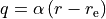 .
See Medvedev and Ushakov J. Quant. Spectrosc. Radiat. Transfer 288, 108255 (2022).
.
See Medvedev and Ushakov J. Quant. Spectrosc. Radiat. Transfer 288, 108255 (2022).
Example:
poten 1
name "X1Sigma+"
symmetry +
lambda 0
mult   1
type   EHH
values
  TE        0.00000000000000E+00
  RE        0.149086580348419329D+01
  AE        0.519274276353915047D+05
  alpha     0.221879954515301936D+01
  c         0.948616297258670499D-01
  B1        0.100084121923090996D+01
  B2        0.470612349534084318D+00
  B3        0.890787339171956738D-01
end
Generic two-state coupled adiabatic potential
Any three single functions implemented in Duo can be used to form a coupled 2x2 system to form PEC with avoiding crossings. This is done using the types Coupled-PEC or COUPLED-PEC-BETA, together with sub-types specifying three functions required to form a coupled system, PEC1, PEC2 and Coupling12. This form also requires that the corresponding numbers of parameters are specified using Nparameters. As above, the last parameter is reserved for the component index (1,2) referring to the adiabatic potential. Here is an example of an adiabatic potential with an avoiding crossing formed from a 2x2 ‘diabatic’ system, an EMO potential, a repulsive potential and an (inverted) EMO used as a coupling (from an AlH model):
poten A
name "A1Pi"
lambda 1
mult   1
type  coupled
sub-types EMO repulsive EMO
Nparameters 13  12 13
values
V0           2.36706506146433e+04
RE           1.64813484193969e+00
DE           50915.756
RREF        -1.00000000000000E+00
PB           4.00000000000000E+00
PU           4.00000000000000E+00
NSPHI        4.00000000000000E+00
NLPHI        4.00000000000000E+00
B0           2.23877956276444e+00
B1           0.000000000000000000
B2          -2.55686572909604e-01
B3           0.00000000000000E+00
B4           0.00000000000000E+00
NREP         11
V0           2.55900000000000E+04
B1           0.00000000000000E+00
B2           0.00000000000000E+00
B3           0.00000000000000E+00
B4           0.00000000000000E+00
B5           0.00000000000000E+00
B6           3.56560923385944e+05
B7           0.00000000000000E+00
B8           0.00000000000000E+00
B9           0.00000000000000E+00
B10          0.00000000000000E+00
V0           6.38813113973348e+03
RE           2.02137412627653e+00
AE           0.000000000000000000
RREF        -1.00000000000000E+00
PB           4.00000000000000E+00
PU           4.00000000000000E+00
NSPHI        4.00000000000000E+00
NLPHI        4.00000000000000E+00
B0           1.84063793349509e+00
B1           0.000000000000000000
B2           3.33171505629389e-03
B3           0.00000000000000E+00
B4           0.00000000000000E+00
COMPONENT    1
end
Here, the keyword sub-type is used to specify the corresponding functions in the form of PEC1 PEC2 COUPLING (COUPLED-PEC) or PEC1 PEC2 BETA (COUPLED-PEC-BETA), where
PEC1, PEC2, COUPLING and BETA are any functions implemented in Duo, e.g. EMO, Lorentzian etc.
In the case of the type COUPLED-PEC, the coupling  is defined explicitly, while for
 COUPLED-PEC-BETA, it is generated using the transformation angle
 :
:
 ,
,
where  and V_2(r) are PEC1 and PEC2, respectively.
An example of the COUPLED-PEC-BETA input for a potential, produced by the coupling of an EMO, REPULSIVE and a diabatic coupling function defined via
the from a Lorentzian form BETA_LORENTZ:
poten A
name "A1Pi"
lambda 1
mult   1
type  coupled-pec-beta
sub-types EMO repulsive BETA_LORENTZ
Nparameters 13  12 2
values
V0           2.36706506146433e+04   fit    (  2.36695116221313e+04)
RE           1.64813484193969e+00   fit    (  1.64805055140387e+00)
DE           50915.756
RREF        -1.00000000000000E+00
PB           4.00000000000000E+00
PU           4.00000000000000E+00
NSPHI        4.00000000000000E+00
NLPHI        4.00000000000000E+00
B0           2.23877956276444e+00   fit    (  2.23878305838811e+00)
B1           0.000000000000000000             (  3.41737763224365e-01)
B2          -2.55686572909604e-01   fit    ( -2.59129061999807e-01)
B3           0.00000000000000E+00
B4           0.00000000000000E+00
NREP         11
V0           2.55900000000000E+04
B1           0.00000000000000E+00
B2           0.00000000000000E+00
B3           0.00000000000000E+00
B4           0.00000000000000E+00
B5           0.00000000000000E+00
B6           3.56560923385944e+05   fit    (  3.56503862575298e+05)
B7           0.00000000000000E+00
B8           0.00000000000000E+00
B9           0.00000000000000E+00
B10          0.00000000000000E+00
gamma        0.025
RE           2.0452
COMPONENT    1.00000000000000E+00
end
Here, the first (lowest) component is produced.
Generic multi-state coupled adiabatic potential
Similarly, a general multi-states adiabatic PEC can be constructed using the sub-type keyword as in the following example:
poten B
name "B2Sig-"
symmetry -
lambda 0
mult   2
type  coupled-pec 3
sub-types EMO REPULSIVE repulsive morse morse morse
Nparameters 9 12 5 5 5 5
values
 VE           3.84687918328484e+04  (EMO)
 RE           1.06429714857428E+00
 AE           9.37229718553690E+04
 RREF        -1
 PL           4.0
 PR           4.0
 NL           0
 NR           0
 B0           1.71356377423284e+00
 NREP         1.10000000000000E+01  (Repulsive)
 VE           2.80256612266818E+04
 B1          -4.80456388326200E+04
 B2           6.81205015447116E+05
 B3          -3.05419508907820E+06
 B4           5.40844612343380E+06
 B5           0.00000000000000E+00
 B6          -1.19338269517479E+07
 B7           1.65813128105902E+07
 B8          -1.03577590530685E+07
 B9           3.17202522138413E+06
 B10         -3.86459936636037E+05
 NREP         4                     (Repulsive)
 VE           2.80256612266818E+04
 B1           0.0
 B2           0.0
 B3           3.00E+06
 TE           1000                  (Morse)
 RE           2.78
 A            0.8
 A0           2.9999e4
 RREF        -1
 TE           1000                  (Morse)
 RE           2.78
 A            0.8
 A0           2.9999e4
 RREF        -1                     (Morse)
 TE           1000
 RE           2.78
 A            0.8
 A0           2.9999e4
 RREF        -1
 COMPONENT    1
 end
Here, the keyword type has an additional parameter of the number of states to couple:
type coupled-pec 3
sub-types lists the 1D functions for each element, Nparameters gives the number of parameters in each object. The last value in the values section is to indicate the state component to output, 1,2 or 3 in this case.
The order of the objects is important. The N diagonal diabatic elements are listed first, followed by the non-diagonal elements in the following order:
 ,
,  , …
, …  ,
,  , …
, …  …,
…,  . In the code (funcitons.f90), this is implemented as follows
! diagonal part
i = 0
do i1 =1,Ndim
   i = i + 1
   N = Nparameters(i)
   v(i1,i1) = function_multi(i)%f(r,parameters(Ntot+1:Ntot+N))
   Ntot = Ntot + N
enddo
! non-diagonal part
do i1 =1,Ndim
   do i2 =i1+1,Ndim
     i = i + 1
     N = Nparameters(i)
     h(i2,i1) = function_multi(i)%f(r,parameters(Ntot+1:Ntot+N))
     Ntot = Ntot + N
   enddo
enddo
Generic two-state coupled adiabatic transition curves (dipoles, spin-orbit, etc)
Similarly to the generic COUPLED-PEC-BETA functional form used to represent adiabatic PECs from diabatic functions, COUPLED-TRANSIT-BETA form is used to create non-diagonal adiabatic transition curves (e.g. dipole) from two diabatic curves and a unitary transformation as follows. Here, only one of the two states (bra or ket) describes a coupled 2-state system, another one is assumed a single state. Any two single functions designed for transition and coupling properties implemented in Duo can be used to form such a coupled representation, while the last one should be a function describing the transformation angle . This form also requires that the corresponding numbers of parameters are specified using Nparameters. As in other similar adiabatic forms,
the last parameter is reserved for the component-index (1,2) referring to the adiabatic state in question. Here is an example of a dipole moment in the adiabatic representation of CH formed from two diabatic bobleroy` DMCs and in the form of a Lorentzian-type form BETA_Lorentz:
dipole X C
name "<X2Pi|DMX|C2Sigma>"
spin   0.5 0.5
lambda  1 0
type  coupled-transit-beta
sub-types bobleroy bobleroy BETA_Lorentz
Nparameters 7 7 2
values
RE           1.4
RREF        -1.00000000000000E+00
P            4
NT           1
B0           0.71
B1           0.09
BINF         0.00000000000000E+00
RE           1.27
RREF        -1.00000000000000E+00
P            5
NT           1
B0           0.85
B1           0.17
BINF         0.00000000000000E+00
gamma        0.2
RE           1.6566449350
COMPON       1
end
Here, the first (lowest) component is produced. The keyword sub-type is used to specify the corresponding functions in the form of DMC1 DMC2 BETA, where DMC1, DMC2 and BETA are any functions implemented in Duo, e.g. boblery, beta_Lorentzian etc. The transformation from  and
and  from
from  and
and  is via the transformation angle is defined as follows
and COMPON =1,2 is to select or , respectively.
Other functional forms
Surkus-polynomial expansion Surkus (BobLeroy)
(alias BobLeroy)
![V(r) = (1-y_p^{\textrm{eq}}) \sum_{i\ge 0} a_i [y_p^{\textrm{eq}}]^i + y_p^{\textrm{eq}} a_{\rm inf},](_images/math/83826b9b89dd29cb2e438644e995598e017675a5.png)
where  is the Surkus variable with

and  is the asymptote of the potential at
  .
.
See also Eq.(36) in R. Le Roy, JQSRT 186, 167 (2017)
Example:
Bob-Rot  1 1
name "<a2Pi|BR|a2Pi>"
spin   0.5 0.5
lambda 1 1
type  BOBLEROY
factor    1.0   (0, 1 or i)
values
 re         0.17700000000000E+01
 rref      -0.10000000000000E+01
 P          0.20000000000000E+01
 NT         0.30000000000000E+01
 a0        -0.63452015232176E+02
 a1        -0.20566444179565E+01
 a2        -0.13784613913938E+02
 a3         0.00000000000000E+00
 ainf      -0.56030500000000E+02
end
Surkus-damp (alias BobLeroy_damp)
Surkus-polynomial expansion with a damping function:
![V(r) = T_{\rm e} + \left[ (1-y_p^{\textrm{eq}}) \sum_{i\ge 0} a_i [y_p^{\textrm{eq}}]^i + y_p^{\textrm{eq}} a_{\rm inf}\right] f^{\rm damp} + t^{\rm damp} (1- f^{\rm damp}),](_images/math/02a8f15bfd613f32b66f793a34a048170ab968ef.png)
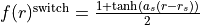
where the damping function is defined by
![f^{\rm damp} = 1-\tanh[\alpha(r-r_0)]](_images/math/848529cb5442dc203bc365886de020de38f0bc9d.png) , and
, and  , and
, and  are parameters.
Example:
Bob-Rot  2 2
name "<a2Pi|BR|+1a2Pi>"
spin   0.5 0.5
lambda 1 1
type  BOBLEROY_damp
factor    1.0   (0, 1 or i)
values
re         0.17700000000000E+01
rref      -0.10000000000000E+01
P          0.20000000000000E+01
NT         0.30000000000000E+01
a0        -0.63452015232176E+02
a1        -0.20566444179565E+01
a2        -0.13784613913938E+02
a3         0.00000000000000E+00
ainf      -0.56030500000000E+02
tdamp      0.00000000000000E+00
r0         0.10000000000000E+01
alpha      0.30000000000000E+01
end
Coxon-type Surkus-polynomial expansion BobCoxon
(alias Bob-Coxon-Surkus)
![`V(r) = (1-y_q^{\textrm{eq}}) \sum_{i=0}^{N} a_i [z_p^{\textrm{eq}}]^i + y_q^{\textrm{eq}} a_{\rm inf},](_images/math/7243a02ab39ffcc4d057564b56efc396890aeae7.png)
where  and
and  are Surkus variables with and two different values of and :
is the asymptote of the funciton at and
See also Eq.(26) in Coxon and Hajigeorgiou, JQSRT 151, 133 (2015)
Example:
BobCoxon  1 1
name "<a2Pi|BR|a2Pi>"
spin   0.5 0.5
lambda 1 1
type  BOBLEROY
factor    1.0   (0, 1 or i)
values
 rref       0.17700000000000E+01
 p          6
 q          2
 NS         2
 NL         3
 a0        -0.63452015232176E+02
 a1        -0.20566444179565E+01
 a2        -0.13784613913938E+02
 a3         0.00000000000000E+00
 ainf      -0.56030500000000E+02
end
POLYNOM_DIMENSIONLESS
This function is a polynomial
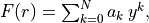 in terms of the dimensionless variable

The order of the parameters in the input is as follows 
Example
dipole 1 1
name "L_2015"
type POLYNOM_DIMENSIONLESS
spin   0.0 0.0
lambda  0  0
values
 re   1.12832252847d0
 a0   -0.1229099d0
 a1    3.604742d0
 a2   -0.23716d0
 a3   -3.67326d0
 a4    1.4892d0
 a5    1.8293d0
 a6   -4.342d0
end
PADE_GOODISMAN2 (PADE2)
![\mu(r) = \left[P(a_i,y) + a_3/2 \right] \frac{z^3}{1+z^7}](_images/math/868bae589e5e0e43ec6aea041f584c459699b7ab.png) ,
,
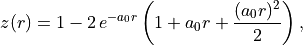
where
 ,
,
 ,
,
and  is a Tchebychev polynomial
  with
with  and a_2 = 1.
See Goodisman, J. Chem. Phys. 38, 2597 (1963).
Example:
dipole  1 1
name "<X,2Pi|DMC|X,2Pi>"
spin   0.5 0.5
lambda  1  1
factor   1   (0, 1 or i)
type       PADE_GOODISMAN2
Values
 RE           1.15078631518530E+00
 B0          -2.36079498085387E+02
 B1           4.85159555273498E+02
 B2          -3.47080753964755E+02
 B3          -2.26690920882569E+02
 B4          -3.56214508402034E+02
 B5          -4.58074282025620E+02
 B6          -4.01237658286301E+02
end
MEDVEDEV_SING2 (SING2)
Dipole moment function:
![\mu(r) = \frac{\left[1-\exp(-r \alpha)\right]^n}{\sqrt{\left(r^2-r_1^2\right)^2+b_1^2} \sqrt{\left(r^2-r_2^2\right)^2+b_2^2}}\sum_{i=0}^kc_i\left(1-2e^{- r\beta}\right)^i](_images/math/bdddea1c1f638e9e9824a315b50381bfc8cd7cb5.png) .
.
Example:
dipole  1 1
name "<X1Sigma+|dmz|X1Sigma+>"
spin   0 0
lambda  0  0
type   MEDVDEDEV_SING2
values
 alpha   0.528882306544608771D+00
 beta    0.174842312392832677D+01
 r1      0.367394402167278311D+00
 b1      0.126545114816554061D+00
 r2      0.226658916500257268D+01
 b2      0.263188285464316518D+01
 n       5
 c0      0.954686180104024606D+04
 c1     -0.100829376358086127D+06
 c2      0.343009094395974884D+06
 c3     -0.593296257373294560D+06
 c4      0.574050119444558513D+06
 c5     -0.296914092409155215D+06
 c6      0.644340312384712088D+05
end
IRREG_CHEBYSHEV_2024
This functional form was introduced by Meshkov et al., Mol. Phys. (2024) as an
irregular analytic representation suitable for permanent dipole-moment curves (DMCs) over a very wide range of
interatomic distances. In Duo it is implemented for generic -dependent fields, and is typically used for
permanent dipoles.
The function is defined as
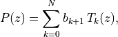
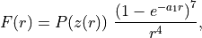
where  are Chebyshev polynomials of the first kind.
The parameters are supplied in the values block as:
a0anda1(real);Chebyshev coefficients
b1, b2, ..., b_{N+1}.
Note
Internally, the Chebyshev series is evaluated using a stable Clenshaw recurrence. The coefficients b1.. correspond
to  in the order written in the input (i.e.
 b1 multiplies  ).
).
Example (permanent dipole moment curve):
dipole  1 1
name "<X1Sigma+|DMZ|X1Sigma+>"
spin   0.0 0.0
lambda  0  0
type   IRREG_CHEBYSHEV_2024
factor   1
values
  a0   2.93767d0
  a1   0.76042d0
  b1     588.66060d0
  b2   -1095.24464d0
  b3    1163.00881d0
  b4   -1020.26040d0
  b5     755.18055d0
  b6    -566.96168d0
  b7     329.26551d0
  b8    -208.85637d0
  b9      89.53594d0
  b10    -46.60804d0
  b11     11.64195d0
  b12     -4.51507d0
end
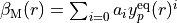
Mass-dependent BOB non-adiabatic Surkus-polynomial expansion BOBNA
BOB-correction.

where is the Surkus variable,  is given by
![t(r) = \mu_a \sum_{i\geq 0} a_i [y_p^{\textrm{eq}}]^i + \mu_b \sum_{i\geq 0} b_i [y_p^{\textrm{eq}}]^i,](_images/math/c39a02593a436bbc8d8071bd1c8d7fda9cfef744.png)
 is the asymptote of the potential at as given by

The mass-dependent factors are given by
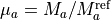
where  and
and  are the reference masses of the parent isotopologue.
Example:
Bob-Rot  1 1
name "<a2Pi|BR|a2Pi>"
spin   0.5 0.5
lambda 1 1
type  BOBNA
factor    1.0   (0, 1 or i)
values
 re         0.17700000000000E+01
 Maref         1.0000
 Ma            1.0000
 Mbref         12.000
 Mb            12.000
 P          0.20000000000000E+01
 NTa        0.30000000000000E+01
 NTb        0.30000000000000E+01
 a0        -0.63452015232176E+02
 a1        -0.20566444179565E+01
 a2        -0.13784613913938E+02
 a3         0.00000000000000E+00
 ainf      -0.56030500000000E+02
 b0        -0.63452015232176E+02
 b1        -0.20566444179565E+01
 b2        -0.13784613913938E+02
 b3         0.00000000000000E+00
 binf      -0.56030500000000E+02
end
SIGMOID function
This form has been initially introduced for the diabatic couplings.
 ,
,
where is expressed in the the Surkus-type expansion
 ,
,
as a simple power series in the reduced variable:

with as an integer parameter. It allows for extra flexibility in the degree of the polynomial on the left or on the right sides of a reference position which we take at . This is specified by the parameters and , respectively.
Example:
diabatic 1 2
name "<a3Piu|diab|b3Piu>"
type  sigmoid
lambda 1 1
mult   3 3
values
Te          0.0
Re          1.31
Ae          500.0
RREF       -1
P           4
b0          2.6
b1          0.0
b2          0.0
b3          0.0.
end
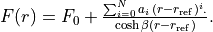
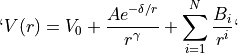
EMO-SWITCH function
This is an EMO form with a short-range finite asymptote built using the sigmoid:

where  and
and  are the corresponding EMO and Sigmoid functions, respectively introduced above and :math:` f_{rm asymptote}` is the constant defining the short-range asymptote.
Example:
spin-orbit 1 2
name "<a2Pi|SO|a2Pi>"
type  EMO-switch
lambda 1 1
mult   2 2
values
   F0           2000.0
   RE           1.1
   AE           0.0000
   RREF        -1.00000000000000E+00
   PL           5.00000000000000E+00
   PR           5.00000000000000E+00
   NL           2.00000000000000E+00
   NR           2.00000000000000E+00
   B0           1.95853328535203e+00
   B1           0.00000000000000E+00
   B2           7.14678340571366e-02
   V0           0.00000000000000E+00
   RE           0.900000000000000000
   A0           1.000000000000000000
   RREF        -1.00000000000000E+00
   P            7.00000000000000E+00
   B0           100
   Blimit        0.00
end
Diabatic/non-adiabatic couplings
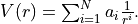
LORENTZ
Alias is LORENTZIAN. A Lorentzian type function used to represent the diabatic coupling:
 ,
,
where
Example:
diabatic A C
name "<A|diab|C>"
lambda 1
mult   2
type  Lorentz
values
 V0           0.000000000000000000
 RE           1.98
 gamma        0.05
 a0           1.58
end
LORENTZ-SURKUS
Alias is LORENTZIAN-SURKUS. A slightly different Lorentzian function combined with a Sukrus expansion as follows:
 ,
,
where
![f_{\rm S}(r) = 1 + \sum_{i=1}^N a_i \left[\frac{(r^p-r_0^p)}{(r^p+r_0^p)}\right]^i.](_images/math/5967135f2a79fd217a19667f3aeea144ff0ed213.png)
Example:
diabatic A C
name "<A|diab|C>"
lambda 1
mult   2
type  Lorentz-Surkus
values
 gamma        0.05
 RE           1.98
 p            4
 a1           0.1
 a2           0.004
end
SQRT(LORENTZ)
Alais SQRT(LORENTZIAN).
A square-root of a Lorentzian type function used to represent the diabatic coupling:
 ,
,
where
Example:
diabatic 3 5
name "<A|diab|C>"
lambda 1
mult   2
type  sqrt(Lorentz)
values
 V0           0.000000000000000000
 RE           1.98
 gamma        0.05
 a0           1.58
end
Generic two-state diabatic coupling using the angle  
As discussed above, a diabatic coupling funciton can be generated from two diabatic PECs and a transformation angle type as given by
,
using the COUPLED-DIABATIC, where can be any function sub-type. For example:
diabatic A C
name "<A|diab|C>"
lambda 1
mult   2
factor 1.0
type   coupled-diabatic
sub-types BETA_Lorentz
factor 1.0
values
gamma        2.75474715845893e-03
RE           2.02
end
is to generate a diabatic coupling generated from PEC A, PEC B (defined in the corresponding POTENTIAL sections) and a BETA_Lorentz function.
Implementation guide
All these analytical functions are programmed as Fortran double precision functions
in the module functions.f90.
Below is an example of a function for the EMO potential energy function.
function poten_EMO(r,parameters) result(f)
  !
  real(rk),intent(in)    :: r             ! geometry (Ang)
  real(rk),intent(in)    :: parameters(:) ! potential parameters
  real(rk)               :: y,v0,r0,de,f,rref,z,phi
  integer(ik)            :: k,N,p
  !
  v0 = parameters(1)
  r0 = parameters(2)
  ! Note that the De is relative the absolute minimum of the ground state
  De = parameters(3)-v0
  !
  rref = parameters(4)
  !
  if (rref<=0.0_rk) rref = r0
  !
  if (r<=rref) then
    p = nint(parameters(5))
    N = parameters(7)
  else
    p = nint(parameters(6))
    N = parameters(8)
  endif
  !
  if (size(parameters)/=8+max(parameters(7),parameters(8))+1) then
    write(out,"('poten_EMO: Illegal number of parameters in EMO, check NS and NL, must be max(NS,NL)+9')")
    print*,parameters(:)
    stop 'poten_EMO: Illegal number of parameters, check NS and NL'
  endif
  !
  z = (r**p-rref**p)/(r**p+rref**p)
  !
  phi = 0
  do k=0,N
   phi = phi + parameters(k+9)*z**k
  enddo
  !
  y  = 1.0_rk-exp(-phi*(r-r0))
  !
  f = de*y**2+v0
  !
end function poten_EMO
To define a new functional form, apart from the actual function, a new reference case identifying this calculation
options needs to be added as part of the case select section in the subroutine define_analytical_field, for example:
case("EMO") ! "Expanded MorseOscillator"
  !
  fanalytical_field => poten_EMO
Glossary
- bob-z-m-switch
Born–Oppenheimer breakdown Z–M switching form (hyphenated alias). Use as
type BOB-Z-M-SWITCH.- bob_z_m_switch
Born–Oppenheimer breakdown Z–M switching form. Use as
type BOB_Z_M_SWITCH.- bobleroy
Le Roy-style BOB function (BobLeroy). Use as
type BobLeroy.- bobleroy_damp
Damped Le Roy-style BOB function (BobLeroy with damping). Use as
type BobLeroy_damp.- bobna
Born–Oppenheimer breakdown (BOB) function of NA type (see section). Use as
type BOBNA.- chebyshev
Chebyshev polynomial expansion in the reduced coordinate. Use as
type Chebyshev.- co_x_ubos
CO X-state UBOS-specific functional form (see section). Use as
type CO_X_UBOS.- cosh-poly
Hyperbolic-cosine polynomial form (cosh + polynomial) for r-dependent fields. Use as
type COSH-POLY.- coupled_emo_repulsive
Coupled EMO + repulsive term functional form. Use as
type COUPLED_EMO_REPULSIVE.- ehh
Extended Hulburt–Hirschfelder (EHH) potential-energy function. Use as
type EHH.- emo
Extended Morse Oscillator potential-energy function. Use as
type EMO.- emo-switch
EMO potential combined with a switching function (EMO-SWITCH). Use as
type EMO-SWITCH.- irreg_chebyshev_2024
Irregular Chebyshev representation introduced by Meshkov et al., Mol. Phys. (2024). Use as
type IRREG_CHEBYSHEV_2024.- irreg_chebyshev_dmc
Irregular Chebyshev representation for dipole-moment curves (legacy name). Use as
type irreg_chebyshev_DMC.- lorentz
Lorentz-type line-shape / damping functional form for r-dependent fields. Use as
type LORENTZ.- lorentz-surkus
Lorentz-type form expressed in a Surkus-mapped coordinate. Use as
type LORENTZ-SURKUS.- m-s
Morse–Surkus (M–S) type functional form (see section). Use as
type M-S.- marquardt
Potential-energy functional form referred to as Marquardt in Duo. Use as
type Marquardt.- medvedev_sing2
Medvedev-style SING2 variant (see section for definition). Use as
type MEDVEDEV_SING2.- mlj
MLJ functional form for r-dependent fields (see section). Use as
type MLJ.- mlr
Morse Long-Range potential-energy function. Use as
type MLR.- mlr_3
Coxon & Hajigeorgiou MLR3 Morse Long-Range potential with Douketis damping. Use as
type MLR_3.- modified-morse
Modified Morse potential-energy function (MMorse-style). Use as
type Modified-Morse.- morse
Morse potential-energy function. Use as
type Morse.- morse_damp
Damped Morse-type functional form (Morse with additional damping/regularisation). Use as
type Morse_damp.- pade2
Pade-type rational functional form (order 2) for r-dependent fields. Use as
type PADE2.- pade_goodisman2
Goodisman-style Pade-type rational functional form (order 2). Use as
type PADE_GOODISMAN2.- polynom_decay_24
Polynomial with decay form introduced/updated in 2024 (see section for definition). Use as
type POLYNOM_DECAY_24.- polynom_decay_damp
Polynomial with exponential decay and damping (see section for definition). Use as
type POLYNOM_DECAY_DAMP.- polynom_dimensionless
Dimensionless polynomial expansion (see section for reduced coordinate). Use as
type POLYNOM_DIMENSIONLESS.- polynomial
Simple polynomial expansion in r (or reduced variable, as defined in the section). Use as
type Polynomial.- repulsive
Repulsive-wall style analytic form for r-dependent fields. Use as
type REPULSIVE.- sigmoid
Sigmoid switching/morphing function used to interpolate between functional forms. Use as
type SIGMOID.- sing2
Singular/irregular functional form (SING2) used for certain r-dependent fields. Use as
type SING2.- spf
Switching/partition (switch) function used to combine fields piecewise. Use as
type SPF.- sqrt_lorentz
Square-root Lorentz-type functional form for r-dependent fields. Use as
type SQRT(LORENTZ).- surkus
Surkus variable / Surkus mapping used to define reduced coordinates. Use as
type Surkus.- surkus-damp
Surkus mapping with additional damping factor. Use as
type Surkus-damp.- two_coupled_bobs
Two coupled BOB functions/fields (see section). Use as
type TWO_COUPLED_BOBS.- two_coupled_emos
Two coupled EMO potentials (coupled-PEC form). Use as
type TWO_COUPLED_EMOS.