Specification of curves and couplings (Duo objects)¶

Once the main global parameters have been specified as described in the previous sections, it is necessary to introduce the PECs and the various coupling curves defining the Hamiltonian. Dipole moment curves (DMCs), which are necessary for calculating spectral line intensities, are also discussed in this section, as well as some special objects which are used for fitting. Each object specification consists in a first part in which keywords are given and a second one (starting from the values keyword) in which numerical values are given; the order of the keywords is not important, except for values. Each object specification is terminated by the end keyword.

Objects of type poten (i.e., PECs, discussed in more detail below) begin with a line of the kind poten N where N is an integer index number counting over potentials and identifying them. It is recommended that PECs are numbered progressively as 1,2,3,…, although this only restriction is that the total number Nmax of PECs should be not less than the total number of states specified by the keywork nstates.

Most other objects (e.g., spin-orbit) are assumed to be matrix elements of some operator between electronic wave functions and after the keyword identifying their type require two integer numbers specifying the two indexes of the two electronic states involved (bra and ket). The indexes are the numbers specified after the texttt{poten} keyword.

Currently Duo supports the following types of objects: potential, spinorbit, L2, Lx, spinspin, spinspino, bobrot, spinrot, diabatic, lambdaopq, lambdap2q, lambdaq, abinitio, brot, dipoletm, nac.

`potential`¶

Alias: poten. Objects of type poten represent potential energy curves (PECs) and are the most fundamental objects underlying each calculation. From the point of view of theory each PEC is the solution of the electronic Schoedinger equation with clamped nuclei, possibly complemented with the scalar-relativistic correction and with the Born-Oppenheimer Diagonal correction (also known as adiabatic correction). Approximate PECs can be obtained with well-known quantum chemistry methods such as Hartree-Fock, coupled cluster theory etc.

Objects of type poten or potential should always appear before all other objects as they are used to assign to each electronic states its quantum numbers. Here is an example for a PEC showing the general structure:

poten 1
name "a 3Piu"
symmetry u
type  EMO
lambda 1
mult   3
values
V0          0.82956283449835E+03
RE          0.13544137530870E+01
DE          0.50061051451709E+05
RREF       -0.10000000000000E+01
PL          0.40000000000000E+01
PR          0.40000000000000E+01
NL          0.20000000000000E+01
NR          0.20000000000000E+01
B0          0.20320375686486E+01
B1         -0.92543284427290E-02
B2          0.00000000000000E+00
end

Here poten 1 refers to the electronic state 1. This label 1 should be used consistently in all couplings as well as in the description of the experimental data.

From 2023, the state labels can be any string of characters, e.g.

poten Ap
name "Ap2Delta"
lambda 2
mult   2
type  EMO
values
V0           1.47069212003828e+04  fit    (  1.47070955806154e+04)
RE           1.817000000000000000
DE           5.92200000000000E+04
RREF        -1.00000000000000E+00
PL           4.00000000000000E+00
PR           4.00000000000000E+00
NL           1.00000000000000E+00
NR           4.00000000000000E+00
B0           1.700000000000000000
B1           0.000000000000000000
B2           0.000000000000000000
B3           0.000000000000000000
B4           0.000000000000000000
end

Integers 1,2,3 from before 2023 will continue working.

`abinitio`¶

Objects of type abinitio (aliases: reference, anchor) are reference, abinitio curves which may be specified during fitting. When they are used they constrain the fit so that the fitted function differs as little as possible from the ab initio (reference). The reference curve is typically obtained by ab initio methods. For any Duo object one can specify a corresponding reference curve as in the following example:

abinitio spin-orbit 1 2
name "<3.1,S=0,0 (B1pSigma)|LSX|+1 (d3Pig),S=1,1>"
spin   0.0 1.0
type   grid
units bohr cm-1
values
 2.3        -3.207178925    13.0
 2.4        -3.668814404    24.0
 2.5        -4.010985122    35.0
 2.6        -4.271163495    46.0
 2.7        -4.445721312    47.0
 2.8        -4.468083270    48.0
end

`Lx` and `L+`¶

Aliases: Lplus, LxLy and L+. It represent matrix elements between electronic states of the molecule-fixed angular momentum operator 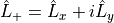$\hat{L}_+ = \hat{L}_x + i \hat{L}_y$ and $\hat{L}_x$ in the $\Lambda$ - and Cartesian-representations, respectively.

`spin-orbit` and `spin-orbit-x`¶

These objects are matrix elements of the Breit-Pauli spin-orbit Hamiltonian in the $\Lambda$ - and Cartesian-representations, respectively.

Example:

spin-orbit  1 3
name "<0,S=0 (X1Sigma+)|LSY|+1 (a3Pi),S=1> SO1"
spin   0.0 1.0
lambda 0 -1
sigma 0.0 -1.0
type   grid
factor sqrt(2)  (1 or i)
units bohr  cm-1
values
  2.80     17.500000
  2.90     15.159900
  3.00     12.347700
  3.10      9.050780
  3.20      5.391190
  3.30      1.256660
  3.40     -3.304040
  3.50     -8.104950
  3.60    -12.848400
  3.70    -17.229100
  3.80    -21.049000
  3.90    -24.250400
  4.00    -26.876900
  4.10    -29.014700
  4.20    -30.756100
  4.30    -32.181900
  4.50    -34.335500
  5.00    -37.348300
end

Here 1 and 3 refer to the electronic states 1 and 3 as introduced using the corresponding potential:

potential 1
name . . .
. . .
end

and


potential 3
. . . . . .
end

From 2023, for the electronic states can be labelled using strings of characters, e.g.

spin-orbit-x  A A
name "<A2Pi|LSZ|A2Pi>"
spin   0.5 0.5
lambda  1  1
sigma  0.5 0.5
units  cm-1
factor    -i   (0, 1 or i)
type polynom_decay_24
<x|Lz|y>  -i -i
values
RE           1.79280000000000E+00
BETA         8.00000000000000E-01
GAMMA        2.00000000000000E-02
P            6.00000000000000E+00
B0           2.06176847388046e+02
B1          -7.04066795005532e+01
B2           0.000000000000000000
B3           0.00000000000000E+00
BINF         220.0
end

where A is the reference label used for the electronic state A2Pi.

For the spin-orbit-x case ( $\Lambda$ -representation), the value of the matrix elements of the $\hat{L}_z$ operator must be specified using the <x|Lz|y> keyword. This representation is designed to work with e.g., the MOLPRO outputs. For $\Lambda\ne 0$ , the diagonal SO-matrix element (e.g. between to $\Pi$ -components of $\Lambda=1$ ) should be specified using the 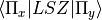$\langle \Pi_x|LSZ |\Pi_y \rangle$ component (e.g. $\langle 1.2 |{\rm LSZ} |1.3 \rangle$ ).

`spin-spin`¶

Parametrised phenomenological spin-spin operator (diagonal and off-diagonal). The diagonal spin-spin matrix elements are given by

$\langle v,S,\Sigma |H^{\rm SS}(r) |v^\prime, S,\Sigma \rangle = \langle v| f_{\rm SS}| v^\prime \rangle \left[ 3 \Sigma^2- S(S+1) \right]$ .

Note

The definition of $f_{\rm SS}$ is different from the spectroscopic spin-spin constant $\lambda$ :

$\langle v| f_{\rm SS}| v^\prime \rangle = \frac{2}{3} \lambda$ .

The non-diagonal spin-spin matrix elements are given by

$\langle v,S,\Sigma |H^{\rm SS'}(r) |v^\prime, S^\prime,\Sigma^\prime \rangle = (-1)^{\Sigma-\Sigma_{\rm ref}} \left(\begin{array}{ccc} S & 2 & S^\prime \\ -\Sigma & \Sigma^\prime-\Sigma & \Sigma^\prime \end{array} \right) / \left(\begin{array}{ccc} S & 2 & S^\prime \\ -\Sigma_{\rm ref} & \Sigma'_{\rm ref}-\Sigma_{\rm ref} & \Sigma_{\rm ref}^\prime \end{array} \right) \langle v,S,\Sigma_{\rm ref} |H^{\rm SS}(r) |v^\prime, S^\prime,\Sigma_{\rm ref}^\prime \rangle$

where $\Sigma_{\rm ref}$ is a reference curve of the projection of spin used to specify the spin-spin field in the Duo input:

$\langle v,S,\Sigma |H^{\rm SS'}(r) |v^\prime, S,\Sigma \rangle = f_{\rm SS'}(r)$

and $f_{\rm SS'}(r)$ is an off-diagonal spin-spin curve, which is usually reconstructed empirically.

An example of the spin-spin input is given by

spin-spin A a
name "<A|SS|a>"
spin   2.5 1.5
factor  1.0
lambda 0 0
sigma 0.5 0.5
type  BOBLEROY
values
RE           0.16500000000000E+01
RREF        -0.10000000000000E+01
P            0.10000000000000E+01
NT           0.20000000000000E+01
B0           0.74662463783234E-01
B1           0.73073583911575E+01
B2           0.00000000000000E+00
BINF         0.00000000000000E+00
end

`spin-rot`¶

The diagonal matrix elements of the spin-rotational operator are given by

$\langle v,S,\Sigma |H^{\rm S-R}(r) |v^\prime, S,\Sigma \rangle = \langle v| f_{\rm S-R}| v^\prime \rangle \left[ \Sigma^2- S(S+1) \right]$ .

The nonzero off-diagonal matrix elements are

$\langle v,S,\Sigma,\Omega |\langle \Lambda | H^{\rm S-R}|\Lambda \rangle (r) |v^\prime, S,\Sigma\pm 1,\Omega\pm 1 \rangle = \frac{1}{2} \langle v| f_{\rm S-R}| v^\prime \rangle \left[ J(J+1)- \Omega(\Omega\pm1) \right]$ .

and

$\langle v,S,\Sigma,\Omega |\langle \Lambda | H^{\rm S-R}|\Lambda\mp1 \rangle |v^\prime, S,\Sigma\pm 1,\Omega \rangle = -\frac{1}{2} \langle v| f_{\rm S-R}| v^\prime \rangle \langle \Lambda | L_{\pm}|\Lambda \mp1 \rangle \left[ S(S+1)- \Sigma(\Sigma\pm1) \right]$ .

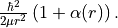
`bob-rot`¶

Alias: bobrot and Alpha. Specifies the (diagonal) rotational $g$ factor (rotational Born-Oppenheimer breakdown term), which can be interpreted as a position-dependent modification to the rotational mass and is introduced as follows

$\frac{\hbar^2}{2\mu r^2} \left(1 + \alpha(r)\right).$

`bob-vib`¶

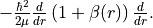
Alias: bobvib and Beta. Specifies the (diagonal) vibrational $g$ factor (Born-Oppenheimer breakdown term), which can be interpreted as a position-dependent modification to the vibrational mass and is introduced as follows

$-\frac{\hbar^2}{2\mu} \frac{d}{dr} \left(1 + \beta(r)\right) \frac{d}{dr}.$

`diabatic`¶

Alias: diabat. Non-diagonal coupling of potential energy functions in the diabatic representation. A diabatic coupling should be centred about the crossing point of the correpsonding diabatic potential curves. For an analitycal (non-grid) representaion, Duo will automatically finds a crossing between the corresponding states and store its value to the second parameter of the diabatic field. It is threfore important to reserve the second line for the reference, expansion point. The search of the crossing point is done by the dividing-by-half approach until the convergence (or 100 iterations) is reached. Only one crossing is currenly supported.

Example:

diabatic  B D
name "<B2Sigma+|DC|D2Sigma+>"
lambda     0 0
spin   0.5 0.5
type  Lorentz
factor    1.0
values
 V0           0.000000000000000000
 RE           2.08                   (this value will be replaced by the actual crossing point between B and D)
 gamma        1.99627265568284e-01
 a            2.75756224068962e+02
 f1           0.000000000000000000
end

Non-adiabatic coupling: `NAC`¶

Non-adiabatic coupling (NAC). It is a non-diagonal coupling element used for adiabatic representation. It appears in the kinetic energy operator as a linear momentum term:

$H^{\rm NAC}_{12}(r) = -\frac{h}{8 \pi^2 c \mu} \left[ -\left(\frac{d^{\gets}}{d r} w^{(12)}- w^{(12)} \frac{d^{\to}}{d r }\right) \right]$ ,

where 12 stands for the coupling between states 1 and 2. By default, a NAC field trigers the “second order NAC” corrections to the corresponding potential energies defined as

$H^{\rm NAC2}_{i}(r) = \frac{h}{8 \pi^2 c \mu} \left(H^{\rm NAC}_{12}(r) \right)^2,$

where $i=1,2$ . In Duo, the diagonal diabatic fields are used to store $H^{\rm NAC2}_{i}(r)$ . If however, the corresponding diabatic fields are directly specified, these second order NAC correction are ignored.

A typical NAC is a Lorentz- or Gaussian-type functions. NAC should be centred about the crossing point of the correpsonding diabatic potential curves.

Example:

NAC  B D
name "<B2Sigma+|NAC|D2Sigma+>"
lambda     0 0
spin   0.5 0.5
type  Lorentz
factor    1.0
values
 V0           0.000000000000000000
 RE           2.08                   (this value will be replaced by the actual crossing point between B and D)
 gamma        1.99627265568284e-01
 a            1.0
 f1           0.000000000000000000
end

The second order NAC corrections can be provided as two diagonal diabatic fields, e.g. (from the YO spectroscopic model)

Example:

diabatic B B
name "<B2Sigma+|NAC2|B2Sigma+>"
lambda     0 0
spin   0.5 0.5
type  grid
factor  1.243548973
values
 1.81020          0.0731621425
 1.81040          0.0735930439
 1.81060          0.0740271189
 1.81080          0.0744643954
 1.81100          0.0749049019
 1.81120          0.0753486669
 1.81140          0.0757957194
 1.81160          0.0762460887
 1.81180          0.0766998042
 1.81200          0.0771568959
 1.81220          0.0776173938
 1.81240          0.0780813285
 1.81260          0.0785487308
 1.81280          0.0790196317
end

diabatic D D
name "<D2Sigma+|NAC2|D2Sigma+>"
lambda     0 0
spin   0.5 0.5
type  grid
factor  1.243548973
values
 1.81020          0.0731621425
 1.81040          0.0735930439
 1.81060          0.0740271189
 1.81080          0.0744643954
 1.81100          0.0749049019
 1.81120          0.0753486669
 1.81140          0.0757957194
 1.81160          0.0762460887
 1.81180          0.0766998042
 1.81200          0.0771568959
 1.81220          0.0776173938
 1.81240          0.0780813285
 1.81260          0.0785487308
 1.81280          0.0790196317
end

Here factor 1.243548973 is $\frac{h}{8 \pi^2 c \mu}$ for YO.

`lambda-opq`, `lambda-p2q`, and `lambda-q`¶

These objects are three Lambda-doubling objects which correspond to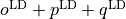: $o^{\rm LD }+p^{\rm LD }+q^{\rm LD }$ , $p^{\rm LD }+2q^{\rm LD }$ , and $q^{\rm LD }$ couplings.

Example:

lambda-p2q  1 1
name "<X,2Pi|lambda-p2q|X,2Pi>"
lambda     1 1
spin   0.5 0.5
type  BOBLEROY
factor    1.0
values
  RE           0.16200000000000E+01
  RREF        -0.10000000000000E+01
  P            0.10000000000000E+01
  NT           0.20000000000000E+01
  B0           0.98500969657331E-01
  B1           0.00000000000000E+00
  B2           0.00000000000000E+00
  BINF         0.00000000000000E+00
end

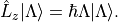
`L2`¶

Alias: L**2. These objects represent matrix elements between electronic states of the molecule-fixed angular momentum operator 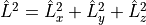$\hat{L}^2 = \hat{L}_x^2 + \hat{L}_y^2 +\hat{L}_z^2$ .

`dipole` and `dipole-x`¶

Dipole (aliases: dipole-moment, TM): Diagonal or transition dipole moment curves (DMCs), necessary for computing (dipole-allowed) transition line intensities and related quantities (Einstein $A$ coefficients etc.).

dipole-x is related to the Cartesian-representation (see below).

`quadrupole`¶

The keyword quadrupole is used to specify transition quadrupole moment curves, which are necessary for computing electric-quadrupole transition line intensities and related quantities. The actual calculation of line strengths requires the quadrupole keyword in the intensity section also (see here).

The quadrupole moment is defined in Cartesian coordinates by the following expression the Shortley convention:

$Q_{\alpha \beta} = -\sum_i e_i \left( r_{i\alpha} r_{i\beta} - \frac{1}{3}r^2_i \delta_{\alpha \beta} \right)$

where $-e_i$ is the charge of the $i-th$ electron with position vector $\vec{r}_i$ . This differs from the Buckingham convention, which is used in many quantum chemistry programs, where:

$Q_{\alpha \beta} = -\frac{3}{2} \sum_i e_i \left( r_{i\alpha} r_{i\beta} - \frac{1}{3}r^2_i \delta_{\alpha \beta} \right)$

Currently Duo requires quadrupole moment curves to be provided in the spherical irreducible representation, with atomic units (a.u.), which can be obtain from the Cartesian components in the Buckingham convention via the relations given by Eq. (6) - (11) of W. Somogyi et al., JCP 155, (2021).

Additionally, the units must be specified via the units keyword. For example

quadrupole 1 1
name "<X3Sigma-|QM20|X3Sigma->"
spin 1 1
lambda 0 0
type grid
units angstrom au
values
 0.8   -1.4747
 0.9   -1.1434
 ...
end

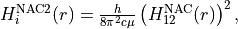
`MAGNETIC`¶

Aliases: MAGNETIC-DIPOLE,``MAGNETIC-X``. Specifies the magnetic dipoles used in magnetic dipole intensity calculations, its electronic orbital angular momentum contribution $\hat{L}_\alpha$ : .. math:

\mu_\alpha = \hat{S}_\alpha + \hat{L}_\alpha,

where $\alpha= x,y,z$ . If Magnetic fields are not provided for magdipole intensity calculations, the corresponding fields Lx are used instead.

`MAGNETROT`¶

Aliases: MAGNETIC-ROT,``MAGNET-ROT``. Specifies the rotational magnetic dipoles used in magnetic dipole intensity calculations. This contribution corresponds to the rotational g-factor, which is the same as the BOB-ROT component. If MagnetRot fields are not provided for magdipole intensity calculations, the corresponding fields Bob-Rot are used instead.

Warning

This feature is currently under construction.

Keywords used in the specification of objects¶

Name and quantum numbers¶

This is a list of keywords used to specify various parameters of Duo objects.

name: object name.

name is a text label which can be assigned to any object for reference in the output. The string must appear within quotation marks. Examples:

name "X 1Sigma+"
name "<X1Sigma\|HSO\|A3Pi>"

lambda: The quantum number(s) $\Lambda$ .

Lambda specifies the quantum number(s) $\Lambda$ , i.e. projections of the electronic angular momentum onto the molecular axis, either for one (PECs) or two states (couplings). It must be an integral number and is allowed to be either positive or negative. The sign of $\Lambda$ is relevant when specifying couplings between degenerate states in the spherical representation (e.g. spin-orbit) Examples:

lambda 1
lambda 0 -1

The last example is relative to a coupling-type object and the two numbers refer to the bra and ket states.

sigma: Spin-projection.

sigma specifies the quantum number(s) $\Sigma$ , i.e. the projections of the total spin onto the molecular axis, either for one (diagonal) or two states (couplings). These values should be real ( $-S\le \Sigma \le S$ ) and can be half-integral, where $S$ is the total spin. sigma is currently required for the spin-orbit couplings only.

Example:

sigma 0.5 1.5

where two numbers refer to the bra and ket states.

mult (alias: multiplicity): Multiplicity

mult specifies the multiplicity of the electronic state(s), given by $(2S + 1)$ , where $S$ is the total spin. It must be an integer number and is an alternative to the spin keyword.

Examples:

mult 3
mult 1 3

The last example is relative to a coupling-type object and the two numbers refer to the bra and ket states.

spin: Total spin.

The total spin of the electronic state(s), an integer or half-integer number. Example:

spin 1.0
spin 0.5 1.5

The last example is relative to a coupling-type object and the two numbers refer to the bra and ket states.

symmetry: State symmetry

This keyword tells Duo if the electronic state has gerade g or ungerade u symmetry (only for homonuclear diatomics) and whether it has positive (+) or negative - parity (only for $\Sigma$ states, i.e. states with $\Lambda=0$ , for which it is mandatory).

Examples:

symmetry +

symmetry + u

symmetry g

The keywords g/u or +/- can appear in any order.

Other control keys¶

type: Type of the functional representaion.

Type defines if the object is given on a grid type grid or selects the parametrised analytical function used for representing the objects or selects the interpolation type to be used. The function types supported by Duo are listed in Duo Functions.

Examples:

type grid
type polynomial
type morse

In the examples above grid selects numerical interpolation of values given on a grid, polynomial selects a polynomial expansion and morse selects a polynomial expansion in the Morse variable. See Duo Functions for details.

Interpolationtype: Grid interpolation

is used only for type grid and specifies the method used for the numerical interpolation of the numerical values. The currently implemented interpolation methods are Cubicsplines and Quinticsplines (default).

Example:

Interpolationtype Cubicsplines
Interpolationtype Quinticsplines

factor: Scaling factor

This optional keyword permits to rescale any object by an arbitrary multiplication factor. At the moment the accepted values are any real number, the imaginary unit $i$ , the square root of two, written as sqrt(2), or products of these quantities. To write a product simply leave a space between the factors, but do not use the * sign. All factor can have a $\pm$ sign. The default value for factor is 1. This keyword is useful, for example, to temporarily zero a certain object without removing it from the input file.

Examples:

factor 1.5
factor -sqrt(2)
factor sqrt(2)
factor 5 i
factor -2 sqrt(2) i

In the last example the factor is read in as $-2 \sqrt{2} i$ . Note that imaginary factors make sense only in some cases for some coupling terms (in particular, spin-orbit) in the Cartesian-representation, see Section~ref{s:representations}.

units

This keyword selects the units of measure used for the the object in question. Supported units are: angstroms (default) and bohr for the bond lengths; cm-1 (default), hartree (aliases are au, a.u., and Eh), and eV (electronvolts) for energies; debye (default) and ea0 (i.e., atomic units) for dipoles; units can appear in any order.

Note

Quadrupole moment curves must be provided to Duo in atomic units, so the units keyword is invalid for these objects.

Example:

units angstrom cm-1 (default for poten, spin-orbit, lambda-doubling etc)
units bohr cm-1
units debye  (default)
units ae0 bohr

<x|Lz|y>, <z|Lz|xy> (aliases <a|Lz|b> and <1|Lz|2>)

This keyword is sometimes needed when specifying coupling curves between electronic states with $|\Lambda| > 0$ in order to resolve ambiguities in the definition of the degenerate components of each electronic state, see:ref:representations.

This keyword specifies the matrix element of the $\hat{L}_z$ operator between the degenerate components of the electronic wave function.

Examples:

<x|Lz|y>   i  -i
<z|Lz|xy> -2i  i

These matrix elements are pure imaginary number in the form $\pm |\Lambda | i$ . It is the overall $\pm$ sign which Duo needs and cannot be otherwise guessed. As shown in the examples above, each factor should be written in the form $\pm |\Lambda | i$ without any space or * sign.

Molpro

A single, stand-alone keywrd to trigger the molpro even for non-x fields.

Example:

molpro

morphing

This keyword is used for fitting and switches on the morphing method.

ZPE: Zero-point-energy

ZPE allows to explicitly input the zero-point energy (ZPE) of the molecule (in cm^-1). This affects the value printed, as by default Duo prints energy of rovibronic levels by subtracting the ZPE. If not specified, the lowest energy of the first $J$ -block (independent of parity) will be used as appear on the line Jlist.

fit_factor

This factor ( $d_{\lambda}$ ) is used as a part of the reference ab initio curves of the abinitio type which (when given) is applied to the corresponding weights assigned to the corresponding values of this object. It is different from fit_factor defined within in Duo fitting.

adjust

This keyword can be used to add a constant value to the values of the potential, which is useful e.g when there is a known systematic error in the values. The keyword is followed by a value and (optionally) units. For a list of the available units see the units keyword above. Note that the units of the shift can be different to the units specified using the units keyword. Default units are cm-1 for PECs, debye for dipole moment curves, and au (atomic units) for quadrupole moment curves.

Examples:

adjust -42 cm-1

adjust

Example:

abinitio poten 1
name "A 1Pi"
type   grid
lambda 1
mult   1
units bohr cm-1
fit_factor  1e1
values
00      32841.37010     0.01
20      17837.88960     0.10
40      8785.33147      0.70
60      3648.35520      1.00
70      2107.10737      1.00
80      1073.95670      1.00
90      442.52180       1.00
00      114.94960       1.00
10      0.00000     1.00
20      48.46120        1.00
30      213.34240       1.00
40      455.16980       1.00
50      739.61170       1.00
60      1038.82620      1.00
70      1332.46170      1.00
00      2059.31119      1.00
50      2619.19233      0.30
00      2682.84741      0.30
00      2554.34992      0.30
00      2524.31106      0.30
00     2561.48269      1.00
00     2575.09861      1.00
end

Cartesian or tensorial representation¶

Internally, Duo represents electronic basis functions in Hund’s case (a), where the electronic function $|\Lambda\rangle$ is an eigenfunction of $\hat{L}_z$ ,

$\hat{L}_z |\Lambda\rangle = \hbar \Lambda |\Lambda\rangle .$

In this Lambda-representation (also referred to as the tensorial representation), the $z$ component is diagonal and carries the signed value $\Lambda$ . Duo therefore stores and manipulates coupling matrix elements and transition moments in this tensorial form. For example, the electronic angular momentum ladder operators are

$\hat{L}_{\pm} = \hat{L}_x \pm i \hat{L}_y ,$

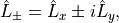
and the spherical (tensorial) components of the body-fixed dipole moment are

$\hat{\mu}_{\pm} = \mp \frac{1}{\sqrt{2}}\left(\hat{\mu}_x \pm i \hat{\mu}_y\right),$

where $\hat{L}_x$ , $\hat{L}_y$ , $\hat{\mu}_x$ , and $\hat{\mu}_y$ are Cartesian components.

Most quantum-chemistry programs (for example Molpro [1]) use real electronic wavefunctions and compute matrix elements of multi-component properties (spin–orbit, electronic angular momentum, dipole moments, etc.) in a Cartesian representation. In this representation, electronic functions are ultimately expressed in terms of real Cartesian components (e.g. [2]) $|x\rangle$ , $|y\rangle$ , $|z\rangle$ , $|xy\rangle$ , etc.

It can be shown that, with appropriate phase choices for the complex Hund’s-case-(a) functions $|{\rm state},\Lambda,S,\Sigma\rangle$ , all coupling matrix elements in the Lambda-representation can be made real. Note that the underlying electronic functions in the Lambda-representation are complex (they contain factors of the form $e^{i\Lambda\phi}$ , where $\phi$ is the azimuthal angle about the molecular $z$ axis).

For that reason, the Lambda-representation is the native representation for Duo. The corresponding input objects assume tensorial components, for example dipole, spin-orbit, L+/L- (and related operators), etc.

Cartesian input¶

Duo can also accept input in the Cartesian representation, which is often the most direct output of quantum-chemistry calculations. In this case Duo assumes that both the electronic wavefunctions and the property operator are given in the Cartesian representation. For many multi-component properties, only one Cartesian component is required (a reference component), since all other non-zero matrix elements can be generated by symmetry/selection rules. Therefore, for Cartesian input Duo typically requires only the x component.

In this case, use the *-x object names, e.g. dipole-x, spin-orbit-x and Lx.

Transformation to the Lambda-representation¶

For Cartesian input, Duo transforms the supplied matrix elements to the Lambda-representation on the fly using a $2\times 2$ unitary transformation,

(1)¶ $|\pm\Lambda\rangle = C_{1}^{\pm|\Lambda|}\,|1\rangle + C_{2}^{\pm|\Lambda|}\,|2\rangle ,$

where $|1\rangle$ and $|2\rangle$ denote the relevant Cartesian components (e.g. $x,y$ or other real combinations such as $xy,\ldots$ ) corresponding to Abelian point-group symmetry pairs (e.g. $A_1,B_1$ or $A_2,B_2$ ). The coefficients $C_{\alpha}^{\Lambda}$ are elements of the unitary transformation from the Cartesian basis to the Lambda-representation.

For non-diagonal spin–orbit couplings with $|\Delta\Lambda|=1$ reported by Molpro, the relevant Cartesian reference matrix element is an $x$ component, e.g. $\langle 1.1 | {\rm LSX} | 1.3 \rangle$ (use spin-orbit-x). In the Lambda-representation the corresponding matrix element acquires a factor of $\sqrt{2}$ .

Note

Do not mix representations within the same object. If the electronic wavefunctions and property are taken from a Cartesian quantum-chemistry calculation, use the corresponding *-x objects consistently (e.g. spin-orbit-x, dipole-x).

Note

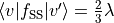
For perpendicular dipole transitions with $|\Delta\Lambda|=1$ , the Cartesian $x$ component (dipole-x), e.g. $\langle 1.1 | {\rm DMX} | 1.2 \rangle$ , has the same numerical value as the tensorial body-fixed component used internally by Duo. The $\sqrt{2}$ factor from the basis transformation is cancelled by the $1/\sqrt{2}$ in the definition of $\mu_{\pm}$ above. Therefore, do not apply any manual $\sqrt{2}$ conversion for dipoles; dipole and dipole-x accept the same numerical values and Duo handles the transformation internally.

Definition of the function or a grid¶

values

This keyword starts the subsection containing the numerical values defining the object. For one of the type``s corresponding to an analytic function, the input between ``values and end contains the values of the parameters of the function. The input consists in two columns separated by spaces containing (i) a string label identifying the parameter and (ii) the value of the parameter (a real number).

In case of fitting (see Duo fitting) a third column should also be provided; the parameters which are permitted to vary during fitting must have in the third column the string fit or, alternatively, the letter f or the number 1. Any other string or number (for example, the string nofit or the number 0) implies the parameter should be kept at its initial value. In the case of fitting, the keyword link can be also appear at the end of each the line; this keyword permits to cross-reference values from different objects and is explained below in this section.

In the case of objects of type grid, the third column can be also used to specify if the grid point needs to vary. The first columns contains the bond length $r_i$ and a second with the value of the object. In the case of object of the abinitio (reference) type and specified as grid a third column can be used to specify the fitting weights (see Duo fitting).

link

This special keyword is used in fitting to force a set of parameters (which may be relative to a different object) to have the same value. For example, in a typical situation one may want to fit a set of PECs and to constrain their dissociation (asymptotic) energy to the same value (because they are expected from theory to share the same dissociation channel).

After the keyword link one should provide three numbers $i_1$ , $i_2$ , $i_3$ defining the parameter ID, where $i_1$ identifies the object type (e.g. poten, spin-orbit, spin-rot etc.), $i_2$ is the object number within the type $i_1$ and $i_3$ is the parameter number as it appears after values. The ID numbers $i_1, i_2, i_3$ are specified in the fitting outputs in the form [i,j,k].

Example of the input:

DE     0.50960000000000E+05   fit     link   1   1   3

Example of the corresponding output

DE     0.50960000000000E+05   [ 1   1   3 ]

Warning

The link feature, where the associated value is replaced with the value the associated parameter is linked to, currently only works when the fitting is on. For all other cases the link keyword is ignored and the actual input value of the given parameter is used, not the one it is linked to. Therefore, to be on the safe side, the correct (fitted) value must be transferred to the place next to the parameter.

Using ab initio couplings in Duo: Representations of the electronic wave functions¶

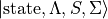
Quantum chemistry programs generally use real-valued electronic wave functions which transform according to the irreducible representations of the C:sub:2v point group (for heteronuclear diatomics) or of D:math:2h (for homonuclear diatomics). On the other hand Duo internally assumes the electronic wave functions are eigenfunctions of the $\hat{L}_z$ operator, which implies they must be complex valued for $|\Lambda| > 0$ . Converting from one representation to the other is simple, as

$|\Lambda\rangle =\frac{1}{\sqrt{2}}\left[\mp |1\rangle - i|2\rangle \right].$

where $1\rangle$ and $2\rangle$ are two Cartesian components of the electronic wave functions in a quantum chemistry program. Duo uses the matrix elements of the $\hat{L}_z$ to reconstruct the transformation between two representations:

The keyword <x|Lz|y> and <z|Lz|xy> (aliases <a|Lz|b> and <1|Lz|2>) is required when specifying coupling curves between electronic states in the MOLPRO representation (spin-orbit-x, Lx and dipole-x) with $|\Lambda| > 0$ in order to resolve ambiguities in the definition of the degenerate components of each electronic state. This is also the value of the matrix element of the $\hat{L}_z$ operator computed for the two component spherical harmonic, degenerate functions $|x\rangle$ and $|y\rangle$ for the $\Pi$ states or $|z\rangle$ and $|xy\rangle$ for the $\Delta$ states etc. The corresponding <x|Lz|y> values for both coupled states must be provided.

Examples:

<x|Lz|y>   i  -i

<z|Lz|xy> -2i  i

This keyword is required for the couplings of the following types: spin-orbit-x, Lx and dipole-x. The suffix -x indicates that Duo expects the x-component (non-zero) of the corresponding coupling.

This keyword should appear anywhere in the object section, before the values keyword.

spin-orbit-x 1 1
name "X-X SO term"
spin 1.0 1.0
lambda 2 2
sigma 1.0 1.0
units angstrom cm-1
type polynomial
factor i
<x|Lz|y>  2i 2i
values
  f 101.2157
end

These matrix elements are pure imaginary number in the form $\pm |\Lambda | i$ . It is the overall $\pm$ sign which Duoneeds and cannot be otherwise guessed. As shown in the examples above, each factor should be written in the form $\pm |\Lambda | i$ without any space or * sign.

Specification of curves and couplings (Duo objects)¶

`potential`¶

`abinitio`¶

`Lx` and `L+`¶

`spin-orbit` and `spin-orbit-x`¶

`spin-spin`¶

`spin-rot`¶

`bob-rot`¶

`bob-vib`¶

`diabatic`¶

Non-adiabatic coupling: `NAC`¶

`lambda-opq`, `lambda-p2q`, and `lambda-q`¶

`L2`¶

`dipole` and `dipole-x`¶

`quadrupole`¶

`MAGNETIC`¶

`MAGNETROT`¶

Keywords used in the specification of objects¶

Name and quantum numbers¶

Other control keys¶

Cartesian or tensorial representation¶

Cartesian input¶

Transformation to the Lambda-representation¶

Definition of the function or a grid¶

Using ab initio couplings in Duo: Representations of the electronic wave functions¶

Table of Contents

Previous topic

Next topic

This Page

Specification of curves and couplings (Duo objects)¶

potential¶

abinitio¶

Lx and L+¶

spin-orbit and spin-orbit-x¶

spin-spin¶

spin-rot¶

bob-rot¶

bob-vib¶

diabatic¶

Non-adiabatic coupling: NAC¶

lambda-opq, lambda-p2q, and lambda-q¶

L2¶

dipole and dipole-x¶

quadrupole¶

MAGNETIC¶

MAGNETROT¶

Keywords used in the specification of objects¶

Name and quantum numbers¶

Other control keys¶

Cartesian or tensorial representation¶

Cartesian input¶

Transformation to the Lambda-representation¶

Definition of the function or a grid¶

Using ab initio couplings in Duo: Representations of the electronic wave functions¶

`potential`¶

`abinitio`¶

`Lx` and `L+`¶

`spin-orbit` and `spin-orbit-x`¶

`spin-spin`¶

`spin-rot`¶

`bob-rot`¶

`bob-vib`¶

`diabatic`¶

Non-adiabatic coupling: `NAC`¶

`lambda-opq`, `lambda-p2q`, and `lambda-q`¶

`L2`¶

`dipole` and `dipole-x`¶

`quadrupole`¶

`MAGNETIC`¶

`MAGNETROT`¶