Duo Input file: general structure¶

The input file is organized in self-contained input lines (e.g.,

atoms  C H

specifies the atoms in the diatomic molecule or in input sections beginning with a specific keyword, e.g., grid and ending with the keyword end:

(Defining the integration grid)
grid
  npoints 501
  range   0.4 8.0
end

Note

The position of the keywords is not important. The input is not key-sensitive, so atoms, ATOMS, Atoms or any other combinations of uppercase and lowercase letters work in exactly the same way.

A comma, a space or a hyphen (minus sign) can all be used as delimiters, so, e.g., one can also

Atoms  C, H

Sometimes keywords have several aliases, which are all equivalent. Lines delimited by parentheses (i.e., round brackets) are ignored and can be used for comments. If in the input there is a line with one of the keyword END, STOP or FINISH all lines after it are ignored.

Most of the input keywords as well as keyword sections can appear in any order, except for Atoms, States/Nstates, POTENTIAL, GRID etc that define other objects and are expected to appear at the top of an input file. In case of a duplicated keyword, the one with the latest appearence takes the presedence.

Here is an example of a Duo inout to compute rovibrational energies of BeH in its ground electronic state using a grid-type potential energy curve by of Jacek Koput, JCP 135, 244308 (2011), Table III (see paper).

 atoms Be H
 (Total number of states taken into account)
 nstates 1

 (Total angular momentum quantum  - a value or an interval)
 jrot 0.5 - 2.5

 (Defining the integration grid)
 grid
   npoints 501
   range   0.4 8.0
   type 0
 end

 CONTRACTION
  vib
  vmax  30
 END


 potential X
 units cm-1 angstroms
 name 'X2Sigma+'
 lambda 0
 symmetry +
 mult   2
 type grid
 values
 0.60     105169.63
 0.65      77543.34
 0.70      55670.88
 0.75      38357.64
 0.80      24675.42
 0.85      13896.77
 0.90       5447.96
 0.95      -1125.87
 1.00      -6186.94
 1.05     -10024.96
 1.10     -12872.63
 1.15     -14917.62
 1.20     -16311.92
 1.25     -17179.13
 1.30     -17620.16
 1.32     -17696.29
 1.33     -17715.26
 1.34     -17722.22
 1.35     -17717.69
 1.36     -17702.19
 1.37     -17676.19
 1.38     -17640.16
 1.40     -17539.76
 1.45     -17142.53
 1.50     -16572.59
 1.55     -15868.72
 1.60     -15063.34
 1.65     -14183.71
 1.70     -13252.86
 1.80       -11313.
 1.90      -9369.74
 2.00      -7518.32
 2.10      -5832.29
 2.20      -4366.71
 2.30      -3155.94
 2.40      -2208.98
 2.50      -1507.72
 2.60      -1013.23
 2.80       -456.87
 3.00       -221.85
 3.50        -72.13
 4.00        -41.65
 4.50         -24.9
 5.00        -14.32
 6.00         -4.74
 8.00         -0.75
 10.00        -0.19
 20.00          0.0
end

Input structure¶

In the following we present the description of the main keywords and options used to define a Duo project. A Duo project file can contain any objectst and descriptors used at different stages of the project. Different keys are used to switch neccesary options on and off.

Structural keywords¶

Atoms: defines the chemical symbols of the two atoms.

Example:

atoms Na-23 H-2

specifies the 23NaD diatomic. Duo includes an extensive database of atomic properties (atomic masses, nuclear spins, isotopic abundances and other quantities) and will use the appropriate values when required. The database should cover all naturally-occurring nuclei as well as all radioactive ones with a half-life greater than one day and is based on the AME2012 and NUBASE2012 databases. Each atom should be specified by its chemical symbol, a hyphen (minus sign) and the atomic mass number, like in the example above. Atomic masses will be used, which is generally the most appropriate choice unless one is explicitely including non-adiabatic corrections. The hydrogen isotopes deuterium and tritium can also be optionally specified by the symbols D and T.

The atomic mass number can be omitted, like in the following example:

atoms Li F

In this case Duo will use the most-abundant isotopes (7Li and 19F in the example above) or, for radioactive nuclei not naturally found, the longest lived one. For example

atoms Tc H

selects for technetium the isotope 97Tc, which is the longest-lived one. A few nuclides in the database are nuclear metastable isomers, i.e. long-lived excited states of nuclei; these can be specified with a notation of the kind

atoms Sb-120m H

In the example above the radioactive isotope of antimony 120mSb is specified (and hydrogen). Another example

atoms Sc-44m3 H

specifies the scandium radioactive isotope 44m3Sc (and hydrogen).

masses:

This is an optional keyword which specifies explicitely the masses of the two atoms (in Daltons, i.e. unified atomic mass units), overriding the values from the internal database if the keyword texttt{atoms} is also specified.

For example, the masses for the CaO molecule would be:

masses 39.9625906 15.99491463

The masses may be atomic masses (the recommended choice if one does not include adiabatic or non-adiabatic corrections), nuclear masses. An up-to-date reference of atomic masses is provided by the AME2012 catalogue (Chin. Phys. C, 36:1603–2014, 2012.) Duo can also make use of position-dependent masses (which is a practical way to account for non-adiabatic effects), see Bob-Rot.

nstates: is the number of potential energy curves (PECs) included in the calculation.

For example, if the ground state and four excited states of a molecule are to be included:

nstates 5

Note that if nstates is set to a number different from the actual number of PECs included in the input file no error message is issued; if more than nstates PECs are included in the input file then the PECs with state > nstates will be ignored. A Duo input file can contain more states and associated objects than required for a current task, with Nstates to specify which states should be used.

Note also that, consistently with the way Duo works internally, nstates is the number of unique PECs in absence of spin-orbit couplings.

An alternative to nstates, the selection of the electronic states can be made via the States list as follows:

States  X A B a C^Pi

where the strings X, A, B, a and C^Pi are also used to label Potential Duo objects to identify the corresponding electronic states:

Potenial X
......
end

Historically, Duo used numbers to label potentials, which is currently extended to simple strings.

For example, to fit the B state only, one should include both the B abd X states (where X is assumed to label the ground electronic state):

States  X B

jrot: specifies the set of total angular momentum quantum numbers to be computed.

These must be integers or half-integers, depending on whether there is an even or odd number of electrons. One can directly specify the values (separated by spaces or commas), specify a range of values (a minimum and a maximum values separated by a hyphen; note than the hyphen must be surrounded by at least by one space on each side). The values do not have to appear in ascending order. For example, the following line

jrot 2.5, 0.5, 10.5 - 12.5,  20.5

specifies the set J = 0.5, 2.5, 10.5, 11.5, 12.5, 20.5.

The first J in the jrot list will be used to define the reference zero-point-energy (ZPE) value for the run.

Note that in the optional sections specifying calculation of spectra (See Intensity) or specifying fitting (section ref{sec:fitting}) is necessary to specify again a list of J values by J and Jlist respectively, which are completely independent from the jrot value specified for energy level calculation.

symmetry: (or Symgroup) is an optional keywork specifying the molecular permutation-inversion symmetry group.

Cs(M) is for heteronuclear diatomics and C2v(M) is for homonuclear diatomics.

For example:

symmetry Cs(M)

Instead of C2v(M) one can write equivalently C2h(M) or G4(M), as these groups are isomorphic; the only difference will be in the labels used for the energy levels. The short-hand notations Cs, C2v, C2h and G4 can also be used and are equivalent to the ones with (M). The energy calculations are done using Cs(M), which is also the default, while for the intensities the C2v(M) group can be also used. Note that this keyword refers to the symmetry of the exact total (electronic, vibrational and rotational) Hamiltonian and not to the $C_{\infty v}$ or the $D_{\infty h}$ point groups, which are relative to the clamped-nuclei electronic Hamiltonian.

Defining the grid¶

grid: specifies an input section with the specifications of the grid of points.

It is used for the solution of the vibrational problem.

Example:

grid
  npoints 501
  range 1.48 , 2.65
end

See Defining the grid

Eigensolver¶

The input section EigenSolver (aliases: FinalStates, diagonalizer, FinalStates) specifies various options relative to the J>0 and/or the coupled problem; it also specifies the LAPACK routine which should be used for matrix diagonalization (both for the solution of the vibrational problem and for the solution of the coupled problem). Example:

Eigensolver
  enermax 25000.0
  nroots 500
  ZPE 1200.0
  SYEVR
END

See Eigensolver: Specifying the eigen-solution of the Hamiltonian.

Vibrational basis and contraction¶

While tje primitive radial basis set is defined by the DVR grid points (see Grid) with the sizes controlled by Npoints, the actual vibratioanl basis set is in the solution of the Schroedinger equation as part of the the rovibronic basis set, is constructed as follows. As a first step the J=0 vibration problem is solved for each electronic state, in which the corresponding Schroedinger equation is solved in the grid representation of npoints. Then a certain number of the resulted vibrational eigenfunctions $|v\rangle$ with $0 \le v\le$ vmax and $\tilde{E} \le$ EnerMax is selected to form the vibrational part of the basis set.

The contraction type is defined in the section CONTRACTION (aliases: vibrationalbasis and vibrations) by the keywords vib (lambda-sigma) or omega.

VibrationalBasis options for the vibrational uncoupled problem
vmax 10 compute vmax vibrational states

end end of vibrational specifications

See Contractions and vibrational basis set.

Duo objects¶

Duo uses concepts of objects or fields of different types to define rhe corresponding curves: potential energy curves (PECs), spin-orbit curves (SOCS), electronic angular momenta curves (EAMs) etc.

For example, potential represents a PEC. From the point of view of theory, each objects, including PEC, is a result of the electronic structure calculation with clamped nuclei, possibly complemented with the scalar-relativistic correction and with the Born-Oppenheimer Diagonal correction (also known as adiabatic correction). Approximate curves can be obtained with well-known quantum chemistry methods such as Hartree-Fock, coupled cluster theory etc and then refined by fitting to the experiment. Some curves are effective objects that can only be defined empirically (e.g. Bob-rot). See Fields for details.

Here is an example for a PEC showing the general structure:

poten 1
name "a 3Piu"
symmetry u
type  EMO
lambda 1
mult   3
values
V0          0.82956283449835E+03
RE          0.13544137530870E+01
DE          0.50061051451709E+05
RREF       -0.10000000000000E+01
PL          0.40000000000000E+01
PR          0.40000000000000E+01
NL          0.20000000000000E+01
NR          0.20000000000000E+01
B0          0.20320375686486E+01
B1         -0.92543284427290E-02
B2          0.00000000000000E+00
end

Duo Fitting¶

Duo allows the user to modify (refine) the potential energy curves and other coupling curves by least-squares-fit to experimental energy term values or wavenumbers. For detaisl see Section Duo Fitting. Teh fitting is activated via the section Fitting, for example:

FITTING
JLIST 2.5,0.5, 1.5 - 11.5, 22.5 - 112.5
itmax 30
fit_factor  1e6
output alo_01
fit_type dgelss
lock      5.0
robust      0.001
energies   (J parity NN  energy ) (e-state v ilambda isigma omega  weight)
 0.5   +   1     0.0000  1  0  0   0.5   0.5    100.000
 0.5   +   2   965.4519  1  1  0   0.5   0.5      7.071
 0.5   +   3  1916.8596  1  2  0   0.5   0.5      5.774
 0.5   +   4  2854.2366  1  3  0   0.5   0.5      5.000
 0.5   +   5  3777.5016  1  4  0   0.5   0.5      4.472
 0.5   +   6  4686.7136  1  5  0   0.5   0.5      4.082
 0.5   +   7  5346.1146  2  0  1  -0.5   0.5    100.000
end

The section can be deactivated by adding the keyword OFF next to FITTING:

FITTING OFF

Intensities and line lists¶

Absorption or emission spectra as well as line lists and other related quantities can be computed by adding an INTENSITY section. For details see Computing spectra (intensities and line lists).

The INTENSITY section can be deactivated by adding the keyword OFF next to FITTING:

INTENSITY OFF

Here is an example of its general structure:

intensity
  absorption
  thresh_intens  1e-15
  thresh_coeff   1e-15
  temperature   300.0
  qstat         10.0
  J,  0.5, 1.5
  freq-window  -0.001,  25000.0
  energy low   -0.001, 6000.00, upper   -0.00, 30000.0
end

Eigenfunctions and reduced density¶

The computed eigenfunctions and radical reduced densities can be printed out into a sperate file (checkpoint). This option can be enabled via the section Checkpoint:

Checkpoint
 density save
 eigenvectors save
 Filename xxxxx
End

See Eigenfunctions and reduced density.

Control keys¶

The following keys can appear anywere in the input file but outsides any sections.

ASSIGN_V_BY_COUNT

(Default) The vibrational quantum number $v$ is assigned by counting the rovibronic states of the same State, $\Lambda$ , $\Sigma$ arranged by increasing energy. The corresponding State, $\Lambda$ , $\Sigma$ labels are defined using the largest-contribution approach (the quantum labels corresponding to the basis set contribution with the largest expansion coefficient). The keyword should appear anywhere in the body of the input file. This is the default option. An alternative is to use the largest-contribution approach also to assign the vibrational quantum number (ASSIGN_V_BY_CONTRIBUTIO), which is used for all other quantum numbers.

ASSIGN_V_BY_CONTRIBUTION

The vibrational quantum numbers is to use the largest-contribution approach also to assign the vibrational quantum number (opposite to ASSIGN_V_BY_COUNT). The largest contribution approach is used for all other quantum numbers.

Print_PECs_and_Couplings_to_File

This keyword will tell Duo to print out all curves to a separate, auxiliary file.

Print_Vibrational_Energies_to_File

This keyword is to print out all vibrational energies into a separate, auxiliary file.

Print_Rovibronic_Energies_To_File

This keyword is to print out all rovibronic energies into a separate, auxiliary file.

DO_NOT_ECHO_INPUT is switch off the printing the inout file at the beginning of the output.
Do_not_Shift_PECs

By default the PECs are shifted such that the minimum of the first PEC is at zero. This leads to Zero-Point-Energy (ZPE) to be defined relative to this zero. All rovibronic energies are by default defined relative to the ZPE. This keyword will suppress shifting PECs so that ZPE is on the absolute scale.

The default is to do the shift of the PECs to the minimum of poten 1. In order to suppress shifting energies to ZPE, use

ZPE 0.0

see also the description of the keyword ZPE.

DO_NOT_INCLUDE_JS_COUPLING

This option is to switch the JS coupling in the Hamiltonian, can be used for debugging purposes.

ASSIGN_V_BY_COUNT

This keyword will switch off the default assigning method (based on the largest basis set contribution) of the vibrational to simple counting of the states, starting from $v=0$ within the same rotational-electronic configuration $|{\rm State}, \Lambda, \Sigma, \Omega \rangle$ . The default method to assign the states with vibrational quantum numbers is known to fail at high excitations.

Legacy

Aliases: Old-Version, Version xxxx (xxxx is the year). This keyword to switch to the original, older version of the molpro function, which was modified in 2019 (bugs fixed and restructured). This keyword should help to reproduce the results published with the old version of the code.

L2Convention

There are two conventions to include the electronic angular momentum $\hat{L}_z^2$ components: it can be defined either as part of the kinetic energy operator (SPECIFY_L^2, SPECIFY_L**2,``Default``) as $\Lambda^2$ or as part of the $\hat{L}^2$ operator (SPECIFY_LX^2_PLUS_LY^2,``SPECIFY_LX**2_PLUS_LY**2``).

Example:

L2Convention SPECIFY_LX^2_PLUS_LY^2

Mem,, Memory: defines the maximal memory (RAM) available for the calculations.

The program will stop with an error if the memory will be acceded before attempting to allocate a new array. The memory can be specified in B, Kb, Mb, Gb or Tb. Example:

64 Gb

SOLUTIONMETHOD * defines the DVR basis set and thus the DVR solution method for the vibrational problem.

Possible methods include 5POINTDIFFERENCES.

SOLUTIONMETHOD  5POINTDIFFERENCES

for the 5 points stencil finite differences to derive the kinetic energy operator. A more efficient method is Sinc DVR (default), which is switched on with

SOLUTIONMETHOD  SINC

Since Sinc is also currently the default method, this does not have to be specified.

Example: computing energy levels (one PEC)¶

Here below there is a commented, minimalistic Duo input file for a single Morse potential; note that the input is case-insensitive. In this particular example we compute the $J=0$ energy levels of a Morse oscillator 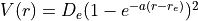$V(r) = D_e (1-e^{-a(r-r_e)})^2$ with $D_e = 40000$ cm^-1, $r_e =1$ Angstrom and $a = 1$ Angstrom $^{-1}$ ; the masses of both atoms are both set to 1 Dalton, so that this example is very approximately corresponds to the hydrogen molecule H:math:_2. The exact energy levels are given by $E_n = \omega (n+1/2) \left[1 - x_e (n+1/2) \right]$ , $n=0, \ldots, 33$ , with $\omega = a \sqrt{2 D_e/\mu} = 2322.593667$ cm^-1 and $x_e = \omega / (4 D_e) = 0.01451621$ .

(DUO test input)
masses 1.00000  1.000000

nstates 1

jrot  0 10

grid
 npoints  250
 range  0.30, 6.50
end

EigenSolver
  enermax  35000.0
  nroots 10
  SYEV
end

VibrationalBasis
  vmax  10
END

poten 1
name "Morse"
type   Morse
lambda 0
mult   1
symmetry +
units  cm-1
units  angstroms
values
 v0   0.000000
 r0   1.000000
 a0   1.000000
 De   40000.
end

The output has this structure:

Input line	Description
(DUO test input)	comment line
masses 1.00000 1.000000	masses of the two atoms, in Daltons**
nstates 1	number of PECs in the input
jrot 0 10	total angular momentum J
grid	specification of the grid
npoints 250	number of grid points
range 0.30, 6.50	$r_\mathrm{min}$ and $r_\mathrm{max}$ , in Angstroms
end	end of grid specification
EigenSolver	options for the Eigensolver
enermax 35000.0	print only levels up to enermax cm^-1
nroots 10	print only nroots lowest-energy levels
SYEV	use SYEV diagonalizer from LAPACK
end	end of input section EigenSolver
VibrationalBasis	options for the vibrational uncoupled problem
vmax 10	compute vmax vibrational states
end	end of vibrational specifications
poten 1	PEC number 1 specification
name “Morse”	label
type Morse	functional form: (extended) Morse function
lambda 0	quantum number $\Lambda$
mult 1	multiplicity, $2S+1$
symmetry +	only for $\Sigma$ terms: $\pm$ symmetry
units cm-1	unit for energies
units angstroms	unit for distances and inverse distances
values	beginning of specification of the parameters
v0 0.000000	specification of global shift
r0 1.000000	specification of $r_e$
a0 1.000000	specification of $a$
De 40000.	specification of $D_e$
end	end of PEC number 1 specification

Duo will by default echo the whole of the input file in the output between the lines (Transcript of the input --->) and (<--- End of the input). This is useful so that the ouput file will also contain the corresponding input. To avoid echoing the input just add the keyword do_not_echo_input anywhere in the input file (but not within an input section).

Duo will then print its logo, the values of the physical constants (used by the program for such things as conversions between different units) and print some of the global input parameters such as the number of grid points, extent of the grid etc.
Duo will then print the values of all objects (PECs, dipole moment curves, couplings) on the internal grid. For PECs Duo will also
compute and print quantities such as the value of the first few derivatives at the minimum, the corresponding equilibrium spectroscopic constants (harmonic frequency, rigid-rotor rotational constant etc.).
Duo will solve the $J=0$ one-dimensional Schroedinger equation for each of the PECs and print the corresponding vibrational (contracted) energies.
Duo will then solve the full problem (with $J >0$ and/or all coupling terms activated). In the example above we specified two values of $J$ , namely $J=0$ and $J=10$ . The $J=0$ energies will be exactly the same as the vibrational (contracted) ones, as in our example there are no couplings at all.

The Duo input files for this example can be found in [Duo Tutorial](https://github.com/Trovemaster/Duo/tree/MOLPRO/examples/tutorial)

See [The ab initio ground-state potential energy function of beryllium monohydride, BeH by Jacek Koput, JCP 135, 244308 (2011)](http://dx.doi.org/10.1063/1.3671610)

The ground electronic state of BeH is a doublet (2Sigma+), see [https://www.ucl.ac.uk/~ucapsy0/diatomics.html](https://www.ucl.ac.uk/~ucapsy0/diatomics.html).

Example: BeH in its ground electronic state¶

In order to solve the nuclear motion Schroediner equation to compute ro-vibronic spectra of BeH with Duo we need to prepare an input file using the following structure (BeH_Koput_01.inp):

 atoms Be H
 (Total number of states taken into account)
 nstates 16

 (Total angular momentum quantum  - a value or an interval)
 jrot 0.5 - 2.5

 (Defining the integration grid)
 grid
   npoints 501
   range   0.4 8.0
   type 0
 end

 CONTRACTION
  vib
  vmax  30
 END


 poten 1
 units cm-1 angstroms
 name 'X2Sigma+'
 lambda 0
 symmetry +
 mult   2
 type grid
 values
 0.60     105169.63
 0.65      77543.34
 0.70      55670.88
 0.75      38357.64
 0.80      24675.42
 0.85      13896.77
 0.90       5447.96
 0.95      -1125.87
 1.00      -6186.94
 1.05     -10024.96
 1.10     -12872.63
 1.15     -14917.62
 1.20     -16311.92
 1.25     -17179.13
 1.30     -17620.16
 1.32     -17696.29
 1.33     -17715.26
 1.34     -17722.22
 1.35     -17717.69
 1.36     -17702.19
 1.37     -17676.19
 1.38     -17640.16
 1.40     -17539.76
 1.45     -17142.53
 1.50     -16572.59
 1.55     -15868.72
 1.60     -15063.34
 1.65     -14183.71
 1.70     -13252.86
 1.80       -11313.
 1.90      -9369.74
 2.00      -7518.32
 2.10      -5832.29
 2.20      -4366.71
 2.30      -3155.94
 2.40      -2208.98
 2.50      -1507.72
 2.60      -1013.23
 2.80       -456.87
 3.00       -221.85
 3.50        -72.13
 4.00        -41.65
 4.50         -24.9
 5.00        -14.32
 6.00         -4.74
 8.00         -0.75
 10.00        -0.19
 20.00         0.0
end

where we use the potential energy curve (PEC) defined in Table III of Koput J. Chem. Phys. 135, 244308 (2011) in a grid form.

An alternative definition is an analytical PEC, see e.g. Barton et. al MNRAS 434, 1469 (2013)

 poten 1
 units cm-1 angstroms
 name 'X2Sigma+'
 lambda 0
 symmetry +
 mult   2
 type grid
 values
 V0             0.00
 RE             1.342394
 DE            17590.00
 RREF         -1.00000000
 PL            3.00000000
 PR            3.00000000
 NL            0.00000000
 NR            0.00000000
 b0            1.8400002
end

Duo Input file: general structure¶

Input structure¶

Structural keywords¶

Defining the grid¶

Eigensolver¶

Vibrational basis and contraction¶

Duo objects¶

Duo Fitting¶

Intensities and line lists¶

Eigenfunctions and reduced density¶

Control keys¶

Example: computing energy levels (one PEC)¶

Example: BeH in its ground electronic state¶

Table of Contents

Previous topic

Next topic

This Page